Excel Scroll and Sort Table

Dashboards have limited space which is why an Excel scroll and sort table is super handy.

Scroll and sort tables allow you to embed an extract of data from a larger table in your Dashboard.

Users can scroll to see all the records and toggle which column to sort by and set the sort order, as shown below:

Download Workbook

Note, this workbook contains functions that are only available to Excel 2021 and 365 users.

Creating an Excel Scroll and Sort Table

Before we had the luxury of Dynamic Arrays, creating an Excel scroll and sort table was a complex task.

It required multiple tables, formulas and helper columns, which I cover in detail in my Excel Dashboard course.

But in this tutorial I want to show you how simple it is to create a scroll and sort table using the new Dynamic Array functions and functionality.

To be clear, the techniques in this tutorial will only work in Excel 2021 and 365 where you have the new Dynamic Array functions.

Source Data

My 20 rows of source data is stored in an Excel Table called ‘Stock’:

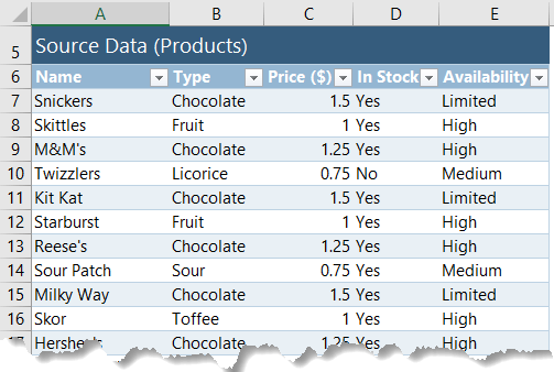
Formatting your data in an Excel Table isn’t strictly necessary, but it makes it quick and easy to write my formulas using the Table’s Structured References.

Excel Scroll and Sort Table Form Controls

The sort column and sort order are controlled using Radio Buttons and I used a Scroll Bar for the scrolling of the table.

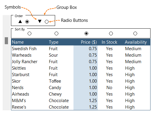
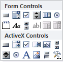
Radio Buttons and Scroll Bars are Form Controls that allow the user to interact with your worksheet.

Note: the up/down triangles are Symbols inserted in the cell.

Form Controls are found on the Developer tab:

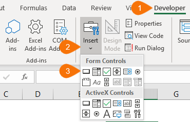
If you don’t see the Developer tab, read this article for instructions how to enable it: Enable the Developer Tab in Excel.

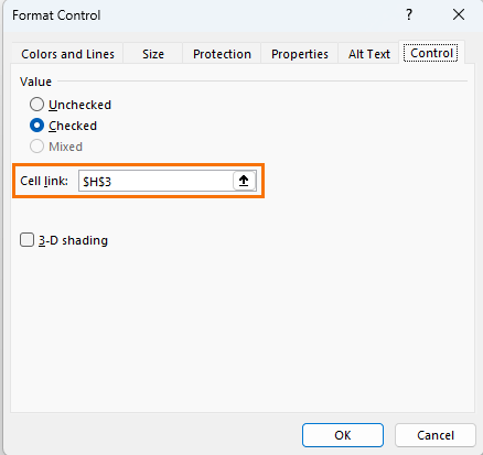
The selection made in a Form Control is returned to a cell that you specify by right-clicking on the Form Control > Format Control > Cell Link:

You can see the Form Control selection results in the image below where the Sort Order button is displayed in cell H3, the Sort By is in cell H4 and the scroll bar position is in cell H5.

These results can also be hidden on another sheet. I've included them beside the table so you can see them in context:

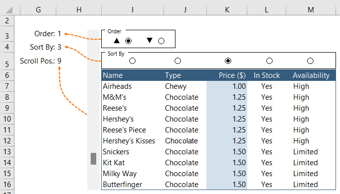
When you place the Radio Buttons inside a Group Box, like I’ve done above, each button is given a number.

For example, the first 'Order' Radio Button is selected and cell H3 contains 1. Likewise, the second 'Sort By' Radio Button is selected and cell H4 contains 2.

The Scroll Bar shows position 9 because it's scrolled almost to the bottom.

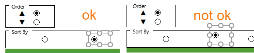
Tip: the whole Radio Button frame must be inside the Group Box for it to form part of the group. If the outer edge of the Radio Button is outside the Group Box, it won’t be included.

Excel Scroll and Sort Table Formula

The table contains a single formula that detects the selections made in the Form Controls and returns an extract of the source data accordingly.

It uses the INDEX, SORT, CHOOSE and SEQUENCE functions. They are linked to named cells for Order (H3), Sortby (H4) and Scroll (H5):

=INDEX( SORT(Stock, SortBy, CHOOSE(Order,1,-1)), SEQUENCE(10,1,Scroll+1,1), {1,2,3,4,5})

In English it reads:

• SORT the tabled called Stock by the 'Sort By' column number displayed in cell H4 named SortBy,
• use CHOOSE* to return 1 for ascending and -1 for descending based on the order specified in cell H3 named Order,
• INDEX the table returned by SORT,
• returning 10 rows starting at the row number in cell H5 named Scroll +1 and increment by 1,
• and return columns 1 through 5.

And because it’s a dynamic array formula it spills the results to create a table 10 rows high and 5 columns wide:

*The SORT function requires 1 for ascending order and -1 for descending order.

The Radio buttons return 1 for ascending and 2 for descending, so we use CHOOSE to return the correct value for the SORT function.

Alternatively you could use SWITCH(Order,1,1,2,-1) to achieve the same result.

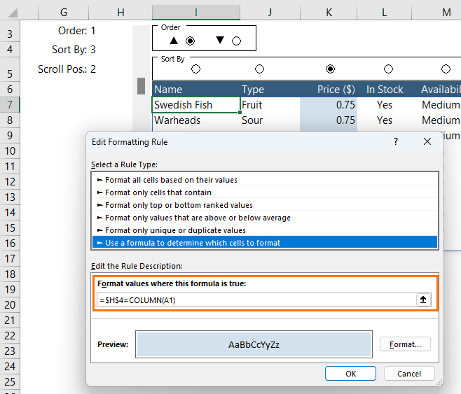
Conditional Formatting

The final touch is to add a conditional formatting formula to highlight the selected ‘Sort by’ column.

Related Tutorials

I realise that you may not have access to dynamic array functions yet, but there are many other ways you can use Form Controls in earlier versions of Excel.

Below are a few tutorials you might like to check out:

	Form Controls
	Toggle Conditional Formatting On and Off using Form Controls
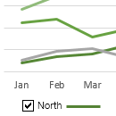	Interactive Excel Charts
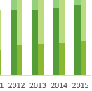	Excel Chart Highlighting

 

Please Share

If you liked this please share this tutorial with your friends and colleagues.