Excel Dynamic Text Labels

I use Dynamic Text Labels all the time, whether it’s in a Dashboard report or chart title, and even to annotate variances like you'll see in this example.

Anyone can create an Excel chart or report but it doesn't mean your reader will get the message you're hoping/trying to convey. With a dynamic text label you can automatically highlight the key points so it's not left to chance.

What is a Dynamic Text Label?

You create Dynamic Text Labels with formulas that join together text and (typically) the result of other nested formulas (the dynamic part). Let’s look at an example.

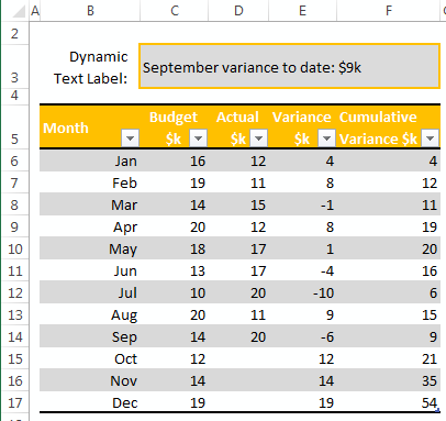
In the image below cell C3 contains my dynamic text label. I used a formula to find the last month in column B that has an Actual value in column D, and the Cumulative Variance from column F, and then constructed the text string you see in cell C3: “September variance to Date: $9k”.

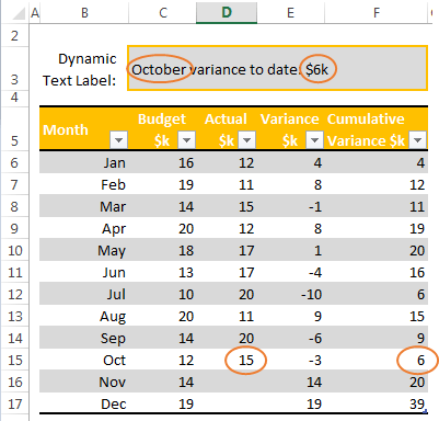
When October actual data is added to the table my dynamic text label will automatically update without me having to do anything:

Download the Workbook

Dynamic Text Labels in Excel Charts

Dynamic text labels are handy in a range of applications. Like I mentioned, I typically use them in report or chart titles, as shown below:

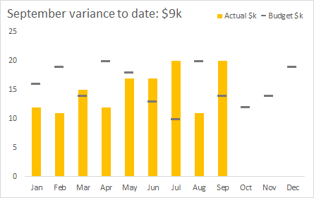
I also like to use them as an alternative to plotting variances on a secodary axis.

An aside; I personally try to avoid secondary axes because they make the chart slower to interpret as the reader has to figure out which series uses which axis.

Link Chart Title to Dynamic Text Label:

1. Add a title to your chart
2. Click on the chart title box
3. While the title box is selected click in the formula bar and type the = sign
4. Click on the cell containing your dynamic label formula with your mouse
5. Press ENTER

Note: You must enter your formula in a cell and then link that cell to the chart title. You cannot put a formula in a chart title, or any other text box or Shape for that matter.

Dynamic Text Label Formula

Here is the formula I used (don’t’ be put off…I’ll explain it 🙂 ):

=TEXT(INDEX(Table1[Month],MATCH(1E+100,Table1[Actual $k],1)),"mmmm")

&" variance to date: "&

TEXT(INDEX(Table1[Cumulative Variance $k], MATCH(1E+100,Table1[Actual $k],1)),"$#,###0k;-$#,##0k"))

Note: the formula above uses Excel Table Structured References instead of regular cell references.

The formula is doing 3 things (hence the colour coding):

1. First it uses INDEX & MATCH to find the name of the month where we have the last Actual value in column D:

TEXT(INDEX(Table1[Month],MATCH(1E+100,Table1[Actual $k],1)),"mmmm")

The MATCH formula looks for value 1E+100, which is scientific notation for a very big number. MATCH will never find that number in the Actual column of my table, and because I’ve set the last argument (match_type) to 1, which means ‘less than’, it simply returns the row number of the last value it does find.

That is, it looks for 1E+100 in column D, it can’t find it so it returns the row number for last value it finds and then INDEX returns the month from column B on that row. See, easy 🙂

Lastly, because the months in column B are actually dates, and in Excel dates are numbers, I need to convert the month returned by INDEX to text because after all, I’m building a text string. So the TEXT function wrapped around INDEX & MATCH tells Excel that I want it to format the date it returns as text, with date formatting “mmmm" applied. This gives me “September”.

2. Next I join the text, “ variance to date: “, using ampersands:

&" variance to date: "&

3. Lastly I use INDEX & MATCH to find the cumulative variance from column F using a similar formula to the first part:

TEXT(INDEX(Table1[Cumulative Variance $k], MATCH(1E+100,Table1[Actual $k],1)),"$#,###0k;-$#,##0k")

Then I wrap INDEX & MATCH in TEXT to tell it that I want the variance figure formatted as $#,##0k, which returns $9k.

And altogether I get:

September variance to Date: $9k

It might seem like a lot of work just to get “September variance to Date: $9k”, but remember we only have to do this once and then next month and the following month it’ll automatically update.

And bear in mind that this dynamic text label has two dynamic parts; the month and the cumulative variance, but they don't have to be this complex so you can modify the formula as required.

Functions Used in this Tutorial

INDEX & MATCH

If you haven’t made friends with INDEX & MATCH yet then I encourage you to master them because once you do you’ll see they’re not that tricky and they open up a lot of Excel opportunities.

TEXT Function

The TEXT function isn’t limited to the examples used here, there is a huge range of applications for it and it’s a great function to have in your Excel tool belt.

Other Ways to Display Variances

Custom Chart Labels

Emoticon Roller Coaster Chart

Please Share

If you liked this or know someone who could use it please click the buttons below to share it with your friends on LinkedIn, Google+, Facebook and Twitter.