• Skip to main content
  • Skip to header right navigation
  • Skip to site footer

My Online Training Hub

Learn Dashboards, Excel, Power BI, Power Query, Power Pivot

  • Courses
  • Pricing
    • Free Courses
    • Power BI Course
    • Excel Power Query Course
    • Power Pivot and DAX Course
    • Excel Dashboard Course
    • Excel PivotTable Course – Quick Start
    • Advanced Excel Formulas Course
    • Excel Expert Advanced Excel Training
    • Excel Tables Course
    • Excel, Word, Outlook
    • Financial Modelling Course
    • Excel PivotTable Course
    • Excel for Customer Service Professionals
    • Excel for Operations Management Course
    • Excel for Decision Making Under Uncertainty Course
    • Excel for Finance Course
    • Excel Analysis ToolPak Course
    • Multi-User Pricing
  • Resources
    • Free Downloads
    • Excel Functions Explained
    • Excel Formulas
    • Excel Add-ins
    • IF Function
      • Excel IF Statement Explained
      • Excel IF AND OR Functions
      • IF Formula Builder
    • Time & Dates in Excel
      • Excel Date & Time
      • Calculating Time in Excel
      • Excel Time Calculation Tricks
      • Excel Date and Time Formatting
    • Excel Keyboard Shortcuts
    • Excel Custom Number Format Guide
    • Pivot Tables Guide
    • VLOOKUP Guide
    • ALT Codes
    • Excel VBA & Macros
    • Excel User Forms
    • VBA String Functions
  • Members
    • Login
  • Blog
  • Excel Webinars
  • Excel Forum
    • Register as Forum Member

Dynamic Dependent Data Validation

You are here: Home / Excel / Dynamic Dependent Data Validation
dynamic dependent data validation
August 26, 2021 by Mynda Treacy

Before we had the luxury of dynamic array functions, creating dependent data validation lists typically required using multiple tables and named ranges, as shown here. Setting them up was laborious, however now that we have dynamic array functions, creating dynamic dependent data validation lists is much easier.

dynamic dependent data validation

Note: this technique requires a Microsoft 365 license for access to dynamic array functions. If you don’t have 365, you can use this technique.

Watch the Video

Subscribe YouTube

Download Workbook

Enter your email address below to download the sample workbook.

By submitting your email address you agree that we can email you our Excel newsletter.
Please enter a valid email address.

Download the Excel Workbook and follow along. Note: This is a .xlsx file please ensure your browser doesn't change the file extension on download.

Dynamic Dependent Data Validation with Dynamic Arrays

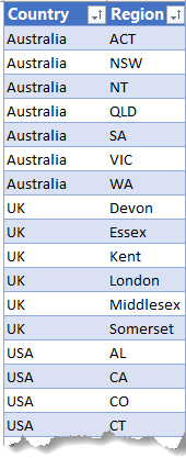
In the table below called TblRegions I have a list of my countries and some of their regions:

Data validation list data

In cell H4 the UNIQUE function extracts a list of sorted country names which are transposed across the columns to form the headers for the region lists:

UNIQUE function extract primary list

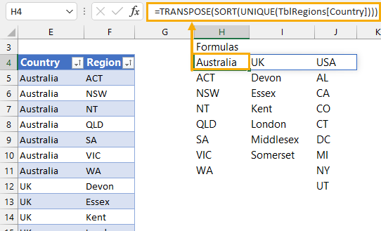
The result of the formula in cell H4 also feeds the data validation list for the countries. Notice the use of the # sign in the Data Validation List cell reference: $H$4# This ensures the data validation list will pick up any new countries added to the TblRegions table.

insert data validation list

In cell H5 the FILTER function returns the list of regions for the country in row 4. I’ve wrapped it in the SORT function to ensure the list returned is sorted alphabetically.

FILTER function extract dependent list

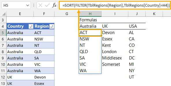
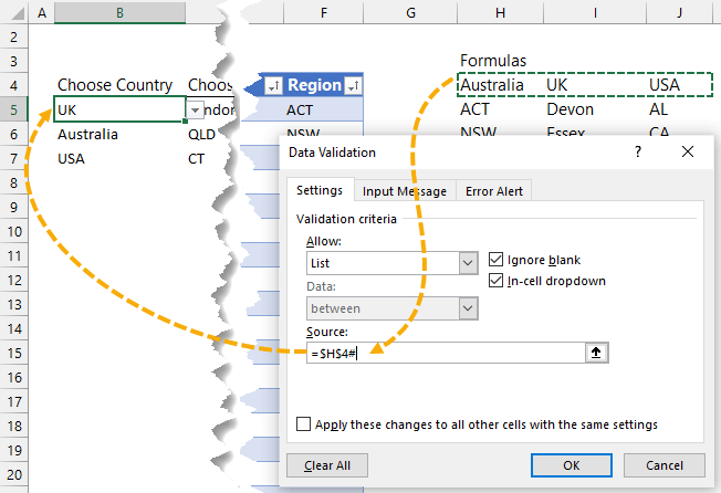
Note: you cannot use the FILTER function directly in the data validation list Source field because this field requires a range as opposed to the array of values returned by FILTER.

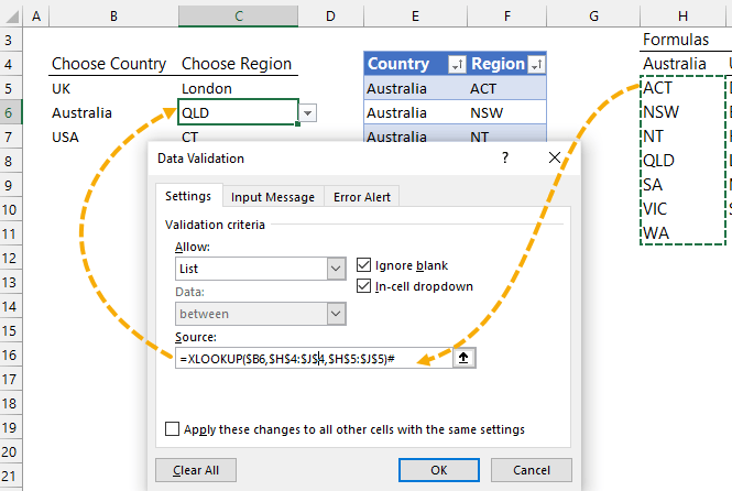
The data validation list uses the XLOOKUP function to return the range containing the list of regions for the country selected in column B. Notice the use of absolute and relative referencing on the lookup column ‘B’ and the use of the # sign to return a dynamic range (watch video for specific instructions):

XLOOKUP function as data validation reference

With this approach any updates to the TblRegions will automatically be included in the data validation lists.

dynamic dependent data validation

More Excel Posts

linear regression

Excel Linear Regression

Excel linear regression is easy with the built-in tools. Use charts to plot linear regression or use the Data Analysis Toolpak.
speed up slow excel files

How to Improve Excel Performance

How to improve Excel performance and the various causes of slow Excel files so you can speed up Excel and avoid problems in future.
Securely Share Excel Files

Securely Share Excel Files

Securely share Excel files stored locally, on OneDrive or SharePoint. Prevent editing or downloading, specify who can open and edit the file.
excel check boxes

Interactive Excel Check Boxes

Excel check boxes are interactive elements you can link to formulas, charts, conditional formatting and more.
tips for working in multiple excel files

Hacks for Working in Multiple Excel Files

Awesome tips for navigating, arranging and working in multiple Excel files. Guaranteed to streamline your workflow and increase productivity.
chatgpt for excel

ChatGPT for Excel

Using ChatGPT for Excel can be hit and miss. Learn the best uses for ChatGPT to make your Excel life easier and what to avoid using it for.
excel templates

Where to Find Free Excel Templates

Where to find free Excel templates and how to create your own Excel templates. Using templates saves time and effort.
Easily Remove Password Protection from Excel Files

Easily Remove Excel Password Protection

How to remove Excel password protection when you’ve forgotten the password. Works for sheets, workbooks and read only files.
Import data from a picture to Excel

Import Data from a Picture to Excel

Import data from a picture to Excel. Works with pictures from a file or the clipboard and loads it to the spreadsheet.
excel online

5 Excel Online Features Better than Desktop

5 Excel Online Features Better than Desktop including searchable data validation, track changes, single line ribbon and more.


Category: Excel
Previous Post:try otherwise power query iferrorIFERROR in Power Query Using TRY OTHERWISE
Next Post:Cool New Features in Excel for Microsoft 365new Excel features

Reader Interactions

Comments

  1. Antonio

    March 15, 2023 at 7:39 pm

    Good Day!
    Firstly allow me to thank you once more for your video and detailed explanation.
    Currently, I have 2 questions I was hoping you would help me with.
    First and the most important question is:
    In your video you’ve described the case when you have countries and regions and how to make them co-dependent.
    What if I would like to add a 3rd column as well?
    So to have a Country column, Region column, and let’s say a City column.
    What I try to achieve is, when I choose a Country, to have accordingly a selection of regions of that country as you already showed us in your video. Then, when I choose the Region, I would like to have on a 3rd column again dependent data of cities, based on the region that I chose.
    Is that possible?
    Ex. I choose Country Greece, then based on this it gives me specific region options in the Region Column and I choose the region Attiki, than based on the Region that I choose in a 3rd column of cities I want to have the options of the cities that are in Attiki region and to choose Athens.
    So 3 columns where each cell depends on the previous one and gives only the options related to the previous column.
    I hope I didn’t describe it too complicated.

    Second Question:
    I did everything step by step as you did in your video and everything worked, however when I create the
    Sort(Filter(Tb1Regions[Region],Tb1Regandions[Country]=H4 and drag it to the right for the other cells to take this formula, it for some reason changes the formula and makes it like this for some reason. Sort(Filter(Tb1Regandions[Country],Tb1Regions[Region]=H4
    SO basically it changes the country and region places inside the formula and I need to manually fix it.
    It however doesn’t change like this for every cell I drag it to, but to every second cell.

    Reply
    • Mynda Treacy

      March 16, 2023 at 10:06 am

      Hi Antonio,

      To answer your first question, yes you can do this by replicating the same steps for the city data. If you’re stuck, please post your question on our Excel forum where you can also upload a sample file and we can help you further.

      To answer your second question, don’t drag to copy. Copy the cell with CTRL+C and then paste the formulas. This will result in the references remaining locked, rather than picking up the next column name.

      Mynda

      Reply
  2. Harshad Nizam

    June 20, 2022 at 3:20 am

    Dear Mam,
    With reference to your video on dependent data validation, i want to ask you a doubt. Since, no one is answering me for that.

    At the video 6min 24 second, you have selected Country as “UK” and Region as “Essex” and other two countries with its Region. Now my doubt or my question is, If I change “UK” to “USA”, then will the region automatically changes or the data validation list changes automatically to “AL” without clicking in region data validation. Beacuse normally it remains under same UK regions when we select Country as USA.
    Please support for my doubt and how to do this. Also, request you to suggest with your best excel courses in linkedin.
    Thanks and Regards,

    Reply
    • Mynda Treacy

      June 20, 2022 at 8:52 am

      Hi Harshad,

      The region does not automatically change if you choose a country that no longer matches the previously selected region. You must click in the region cell and choose a new region. The data validation list will be updated to show regions that match the now selected country. You can download the example file above and try it yourself and you’ll see.

      I don’t put my courses on LinkedIn. You can see my course options here.

      Mynda

      Reply
  3. J-R

    August 30, 2021 at 9:08 pm

    Hi
    for the first method,you can in the data validation box use =indirect(“country[Country]”). -> (“tableName[columnName]”)
    So you don’t need to set the named range.

    Reply
    • Mynda Treacy

      August 31, 2021 at 3:42 pm

      Yep, nice tip! Thanks for sharing. I tend to avoid INDIRECT because it’s volatile, but if used sparingly it’s fine.

      Reply
  4. Guenther Wagner

    August 26, 2021 at 10:57 pm

    Hello,

    if you enter another country, the “2nd” Dropdown list *does not expand*, so only the first dropdown is dynamic…. It still only refers to columns H to J in your example file, the new column (K) is not included….This is a waste of time and useless, please propose a solution where the “secondary” (or dependant() dropdowns for a 4th country also work!
    🙁

    Reply
    • Mynda Treacy

      August 31, 2021 at 4:03 pm

      Hi Guenther,

      To dynamically expand the regions for more countries, copy the FILTER function across more columns and use the ‘not found’ argument in FILTER to return blank with two double quotes, e.g.:
      =SORT(FILTER(TblRegions[Region],TblRegions[Country]=H4,””))

      Then modify the XLOOKUP to also include further columns e.g. if your FILTER formulas are in columns H:P your XLOOKUP would be:
      =XLOOKUP($B5,$H$4:$P$4,$H$5:$P$5)#

      Mynda

      Reply

Leave a Reply Cancel reply

Your email address will not be published. Required fields are marked *

Current ye@r *

Leave this field empty

Sidebar

More results...

Featured Content

  • 10 Common Excel Mistakes to Avoid
  • Top Excel Functions for Data Analysts
  • Secrets to Building Excel Dashboards in Less Than 15 Minutes
  • Pro Excel Formula Writing Tips
  • Hidden Excel Double-Click Shortcuts
  • Top 10 Intermediate Excel Functions
  • 5 Pro Excel Dashboard Design Tips
  • 5 Excel SUM Function Tricks
  • 239 Excel Keyboard Shortcuts

100 Excel Tips and Tricks eBook

Download Free Tips & Tricks

Subscribe to Our Newsletter

Receive weekly tutorials on Excel, Power Query, Power Pivot, Power BI and More.

We respect your email privacy

239 Excel Keyboard Shortcuts

Download Free PDF

mynda treacy microsoft mvpHi, I'm Mynda Treacy and I run MOTH with my husband, Phil. Through our blog, webinars, YouTube channel and courses we hope we can help you learn Excel, Power Pivot and DAX, Power Query, Power BI, and Excel Dashboards.

Blog Categories

  • Excel
  • Excel Charts
  • Excel Dashboard
  • Excel Formulas
  • Excel PivotTables
  • Excel Shortcuts
  • Excel VBA
  • General Tips
  • Online Training
  • Outlook
  • Power Apps
  • Power Automate
  • Power BI
  • Power Pivot
  • Power Query
microsoft mvp logo
trustpilot excellent rating
Secured by Sucuri Badge
MyOnlineTrainingHub on YouTube Mynda Treacy on Linked In Mynda Treacy on Instagram Mynda Treacy on Twitter Mynda Treacy on Pinterest MyOnlineTrainingHub on Facebook
 

Company

  • About My Online Training Hub
  • Disclosure Statement
  • Frequently Asked Questions
  • Guarantee
  • Privacy Policy
  • Terms & Conditions
  • Testimonials
  • Become an Affiliate

Support

  • Contact
  • Forum
  • Helpdesk – For Technical Issues

Copyright © 2023 · My Online Training Hub · All Rights Reserved. Microsoft and the Microsoft Office logo are trademarks or registered trademarks of Microsoft Corporation in the United States and/or other countries. Product names, logos, brands, and other trademarks featured or referred to within this website are the property of their respective trademark holders.