We can use a data validation list or a Slicer to lookup pictures in Excel. This ability to lookup pictures is handy for returning images of products, employees, logos etc. The only limit is your imagination.
In this example I’m going to lookup pictures of the Tour de France stage profiles*.

*Source 2013 Tour de France.
Download Workbook
Enter your email address below to download the sample workbook.
Watch the Video

Lookup Pictures in Excel – Setup
Step 1: Insert the images in a cell
Place each image in its own cell. It’s important that the cell containing the image is at least as big or slightly larger than the image itself. You can see in the screenshot below that the image fits perfectly inside of cell A1.
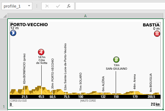
Important: If any part of your image sits outside of the cell it will be distorted when you look it up.
Step 2: Name the image cells
Next, give each cell that contains an image a unique name. You can see in the name box in the screenshot below that the cell is called ‘profile_1’:
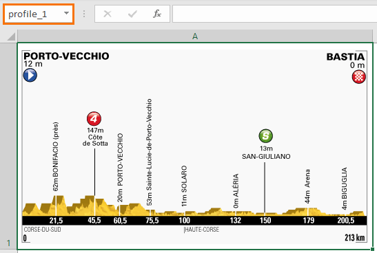
To name a cell, click in the name box (shown in image above), type in the name and press ENTER.
Note: The cell names cannot contain any spaces.
Step 3: Supporting Data
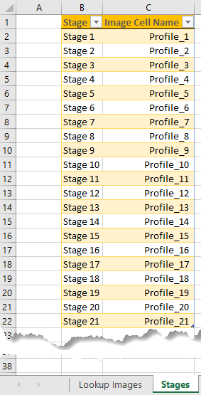
Create a table that lists the images cell names and the name you want to use to lookup the image. You can see my table below (called Table1) contains the list of Stages and the Image Cell Names for each stage.
Tip: If your image name and lookup names are the same then you only need one column.
Step 4: Insert a Data Validation List or Slicer
Next you need to decide how you want your users to lookup the images. In the sample file I’ve included two options, one using a Data Validation List and another using a Slicer.
Data Validation
In the image below in cell B5 I have a data validation list, which is linked to the Stage column of the table shown in step 3.
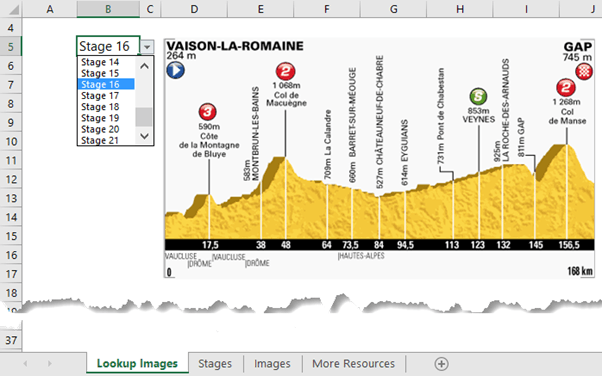
The Stage name in cell B5 returned by the data validation list needs to be converted into the cell name for the image. I’ve used the XLOOKUP function in cell B6 to lookup the Table in step 3, but you could equally use VLOOKUP or INDEX & MATCH:
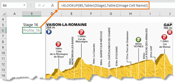
Tip: You can hide this formula on another sheet out of sight. I’ve included it here so you can see it in context.
Slicer
Alternatively, insert a PivotTable based on the Table in step 3. You can see below that mine includes the Stage and Image Cell Name fields and a Slicer for the Stage:
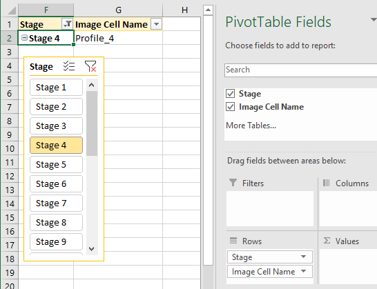
Tip: Cut and paste the Slicer to the sheet where you want the pictures displayed.
As the Slicer selections are made, the PivotTable filters to show the Image Cell Name for the selected stage.
Step 5: Set Up the INDIRECT Named Formulas
Create a named formula using the INDIRECT function that references the cell containing the image cell names returned by the data validation list or the Slicer. In the screenshot below you can see the data validation method named formula is called profile_dv and for the Slicer it’s called profile_slicer:
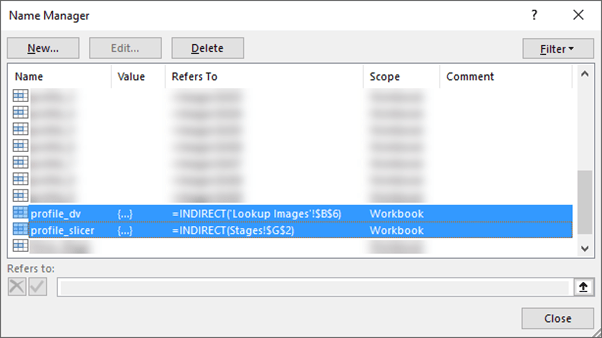
The named formula, profile_dv, references cell B6 on the Lookup Images sheet. And named formula, profile_slicer, references the image cell name displayed in the PivotTable on sheet ‘Stages’ in cell G2.
Step 6: Insert the Image
Copy one of the images and place it on the worksheet where the data validation list or Slicer are that your user will be making their selections from.
With the image selected, click in the formula bar and type an equal sign followed by the named formula you set up in the previous step, then press ENTER:
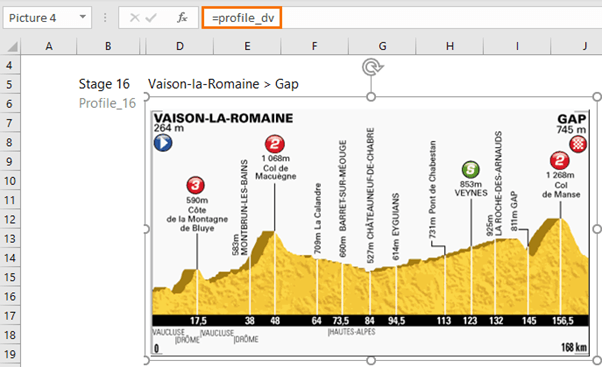
That’s it, you can now lookup Pictures in Excel via the data validation list or Slicer, depending on which method you chose.


Lookup Pictures in Excel. Hello, I have followed the demo and tried six times but I cannot get it to work. Firstly I use VLOOKUP as I don’t have XLOOKUP. The problem is not here. I get to the last process which is clicking on the image and entering the formula name, this gives me the error “Reference is not Valid” I have checked and rechecked.
Hi Anton,
Please post your question on our Excel forum where you can also upload your Excel file and we can help you further.
Mynda
thank you! quick quesiton please, is there a way of making this happen in Excel Online?
(The sheet will ultimately embedded in a webpage so would be great to have this function compatible with Excel Online.)
Last time I checked, objects weren’t available in Excel Online, so possibly not, but things might have changed since then. You can easily test it by saving the file to your OneDrive and opening it in Excel Online.
Thank you so much for this tutorial. Just what I needed. The image lookup works as expected, however the scale of the image changes after selecting a new item from the drop down. “Size” of the picture box stays the same, but I am only seeing the upper corner of the image. I am working on a MacBook Pro, I was thinking maybe resolution of the images is different than my screen? I also downloaded your files and see the same effect. Instead of the entire profile, just the upper left corner.
Hi Karen, as per my reply to the same comment on YouTube: I’d have thought it was because the source image isn’t in a single cell, but if it’s happening in my file as well as yours then I’m not sure why that would be, sorry.
On step 5, where do you put this Indirect function (which cell)?
Hi Debbie, the INDIRECT formulas are set up as named formulas in the name manager: Formulas tab > Define Name.
another perfect explained workshop for using excel in my own workbook.
Cheers, Steven! Glad you found it helpful 🙂
Another great vid, Mynda! 2 quick questions:
1. How did your slicer come out in natural order instead of “Excel order” (1, 10, 11, 12…..). Did you create a custom sort in advance?
2. Could you use the table slicer instead of creating a PT?
Thanks!
Hi Jerry,
Yes, I used a custom list to sort the Slicer 😉
If you assign the Slicer to filter the table then you also need to write another formula to find which row in the table is now visible for the INDIRECT function to reference. Because of this I found it easier just to insert a PivotTable. Call me lazy 🙂
Mynda
great idea once again Mynda,
another Tip:
when dragging pictures to a cell, hold the alt-key and it will snap to the gridlines and be guaranteed to fit exactly
I’ve done a similar thing (in effect, not execution) whereby you can assign a picture to a cell comment’s background format; so that merely hovering over a cell will reveal the image (it was an employee contact list and hovering over an entry showed that person’s picture) – many years ago, before pivots, slicers or even tables
– or XLOOKUP, which I’m now delighted to have and play with too!
jim
Thanks, Jim!
Alt will work as long as the image and cell size are identical (or almost identical), otherwise the image will be aligned to the top left of the cell. This may or may not be an issue when you do the lookup as it’ll depend on how much white space you have around the image and how you want to align it on the lookup sheet.
I remember the comment background image too 🙂 Unfortunately you can’t do it with the new Threaded Comments.
Mynda
I was thinking of dragging opposite corners in turn rather than dragging the whole image, but that risks getting a skewed image (though with even-sized rows the images would all be the same size, which looks better when you select them – if you’re the sort of person who gets obsessed with such fine detail)
I haven’t found the need to use Threaded Comments yet – I still do Notes as they’re now called, I just hope they’ll still be supported (I prefer to keep things simple)
Another picture-based spreadsheet I made used HYPERLINK to open selected images, but that was a little more convoluted and didn’t always work very well
jim
Ah, great idea for charts or other shapes though, as they won’t get distorted.
I love it!
Thanks a bunch
🙂 you’re welcome!
Hi Mynda, thank you for another great video and all the great content you post. I have previously wondered about the uses of INDIRECT and was reminded about it by this video. Its probably a very silly question and I confess to not having played around to test it, but anyway…
… Why do you have to use INDIRECT to reference the cells with the picture name. Why can’t you just use the cell name or reference itself, without the formula wrap around? I’ve always been puzzled by this whenever I see INDIRECT used. Is there a video you could point me to that explains it?
Thanks,
Si
Thanks, Simon.
To answer your question, you can link the picture directly to the named cell e.g. =profile_1 What you can’t do is link the picture to a cell that contains a formula that returns profile_1 i.e. you can’t link the picture to cell B6. You need INDIRECT to tell Excel to use the name in the cell, rather than the underlying formula. More on how INDIRECT works here.
Mynda
File is corrupted and can not be opened.
Hi VJ,
I can’t reproduce that error. It opens fine for me when I download it from the link above. Please try a different browser, or try downloading it again. If you still have problems, please email us and we’ll send you the file.
Cheers,
Mynda
Worked in a different browser, thank you!