Highlight Cells Referenced in Excel Formulas

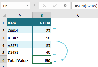
In an ideal spreadsheet our formulas would always reference adjacent cells and columns and it would be obvious which cells contributed to a result, like this:

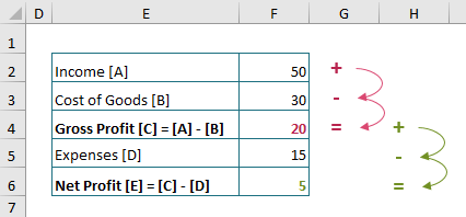
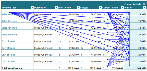
However, in financial modelling and reporting it’s often less obvious, like the example below:

Let’s look at some ways we can easily identify which cells contribute to a result.

Download the Workbook

Trace Precedents and Dependents

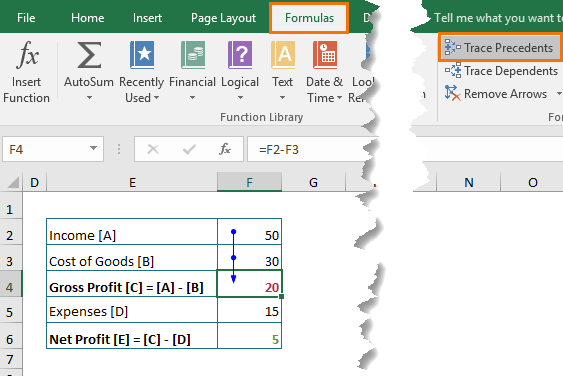
We can use tools like Trace Precedents and Dependents (on the Formulas tab of the ribbon) to get a visual indication of what cells are involved in a formula. For example, in the image below we can see Trace Precedents arrow for cell F4:

And here is the Trace Dependents arrow for the same cell:

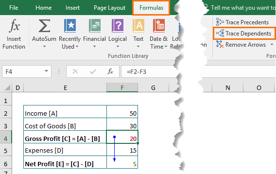
These arrows can be turned off by clicking the ‘Remove Arrows’ button on the Formulas tab.

Trace precedents and dependents arrows are useful for reasonably simple formulas, but they can quickly turn into pick-up sticks in more complex scenarios:

Another easy way to highlight cells referenced in a formula is to press F2 to edit the cell containing the formula in question. With this technique you get a nice color coded visual of the cells involved:

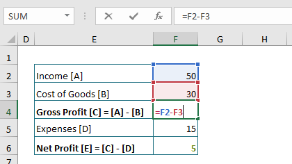
But that’s only good for one cell at a time.

Highlight Cells Referenced in Formulas with Conditional Formatting

Another tool we can use in Excel 2013 and 2016 is Conditional Formatting, it also comes with limitations, but first let’s look at the application.

In the image below, you can see the cells in column C that relate to the totals in cells C12 and C13 by way of color coding:

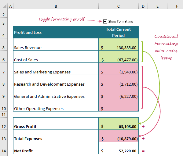
It gives a quick visual check that you can toggle off by unchecking the ‘Show Formatting’ button:

Note: This is quite advanced but if you take your time and refer to the workbook I’m confident you can grasp it.

For this technique we use a Conditional Formatting formula to check if any cells in C5:C10 are referenced in the formula in cell C12.

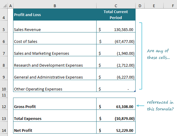
If they are, the cell fill color is set to green. We repeat for the formula in cell C13 and format in pink.

These conditional formatting formulas use the following functions (it looks like a long list, but don’t be put off):

• SEARCH(find_text, within_text, [start_num]) – returns the numeric starting position of text within text.
• ADDRESS(row_num, column_num, [abs_num], [a1], [sheet_text]) – creates a cell reference as text
• ROW([reference]) – returns the row number of a cell reference
• COLUMN([reference]) – returns the column of a cell reference
• FORMULATEXT(reference) – returns the formula as a string/text
• SUBSTITUTE(text, old_text, new_text, [instance_num]) – replaces existing text with new text

Tip: Function arguments in square brackets are optional. E.g. [start_num] in the SEARCH function is an optional argument, meaning you can simply omit it.

Here is the conditional formatting formula we’ll use to check if any of the cells in the range C5:C10 are referenced in the formula in cell C12 (which is =C5+C6):

=SEARCH(ADDRESS(ROW(C5),COLUMN(C5),4,1),FORMULATEXT($C$12))

In English it reads, search the formula contained in cell C12 for the address of the cell at the intersection of ROW 5 and COLUMN C and make it a relative cell reference*. i.e. search for cell reference “C5“ in the formula in cell C12.

*we want relative references because that’s the format of the cell references in the formula in cell C12. More on that soon.

You can see the result below after the ADDRESS, ROW, COLUMN and FORMULATEXT functions are evaluated against cell C5:

=SEARCH("C5","=C5+C6")

And from here we can see that the text, C5, starts at the 2^nd character in the string, =C5+C6, so SEARCH returns 2.

Note: Conditional formatting will be applied when a formula evaluates to any number other than zero, so in this case the formatting is applied.

Handling Absolute References

But what if the formula in C12 contains absolute references, or what if someone thinks they’ll be “helpful” and they later add them?

Well, then we should make this formula more robust so it can handle this scenario. We’ll use the SUBSTITUTE function to replace any dollar signs found in the formula text with nothing, effectively converting any absolute references back to relative references.

=SEARCH(ADDRESS(ROW(C5),COLUMN(C5),4,1),SUBSTITUTE(FORMULATEXT($C$12),"$",""))

Now if anyone changes the formula in cell C12 to contain absolute references they’ll be ignored when the conditional format formula is evaluated.

Alternatives to ADDRESS

A word on the ADDRESS function; we use the ADDRESS function to return the cell reference for each cell we want to check in the range C5:C10. With this formula structure we can apply the conditional format across a range of columns and ADDRESS will dynamically return the correct cell without any modifications.

However, if you just want to check one column, for example column C, then you can simply build your cell reference by concatenating ‘C’ to the ROW function like this:

=SEARCH("C"&ROW(C5),SUBSTITUTE(FORMULATEXT($C$13),"$",""))*$E$3

Alternatively, you could use the CELL function instead of ADDRESS, like so:

=SEARCH(CELL("address",C5),FORMULATEXT($C$13))*$E$3

It’s a bit more succinct, but the CELL function returns an absolute reference so you’d be wise to strip out the $ signs with SUBSTITUTE here too to avoid inconsistencies in the references:

=SEARCH(SUBSTITUTE(CELL("address",C5),"$",""), SUBSTITUTE(FORMULATEXT($C$13) ,"$",""))*$E$3

And now it’s not really any better than the original formula.

Set up the Toggle Excel Party Trick

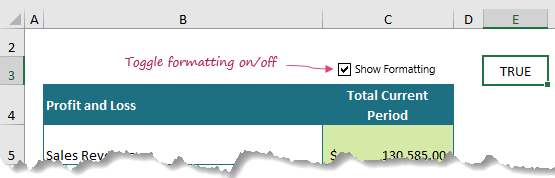
To implement the formatting on/off toggle we simply multiply the formula by the TRUE/FALSE returned by the ‘Show Formatting’ check box form control in cell E3 shown in the image above:

=SEARCH(ADDRESS(ROW(C5),COLUMN(C5),4,1),SUBSTITUTE(FORMULATEXT($C$12),"$",""))*$E$3

Tip: When you perform a math function on TRUE or FALSE they are converted to their numeric equivalents of 1 and 0. So by multiplying the formula by FALSE we’re effectively multiplying by 0, and anything multiplied by 0 = 0, so the Conditional Formatting is not applied.

Learn how to toggle Conditional Formatting on/off.

Conditional Formatting Limitations

1. The Conditional Formatting technique only works with formulas that individually reference cells, i.e. won’t work with a range e.g. =SUM(A1:A5) but will work with =SUM(A1,A2,A3,A4,A5)
2. It only works with Excel 2013 or later as it requires the FORMULATEXT function which was new in Excel 2013.

Related Lessons

• Setting up Conditional Formatting using formulas
• Absolute and Relative References
• Toggle Conditional Formatting On/Off
• SEARCH Function
• CELL Function
• Form Controls