Phil plays 6 a-side football (soccer) in a Supa-Oldie league. They’re all over 35 and that’s considered supa-old in football! Personally I think it’s an excuse to have a beer with the lads, anyway…
Darryl, the fellow who updates the scores, explained to Phil that every week it was taking him 2 hours to prepare the league tables as he had to re-calculate all the stats in his Excel spreadsheet. TWO HOURS!
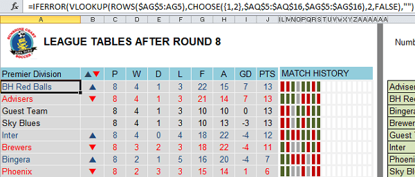
Here is the ‘Before’ photo:
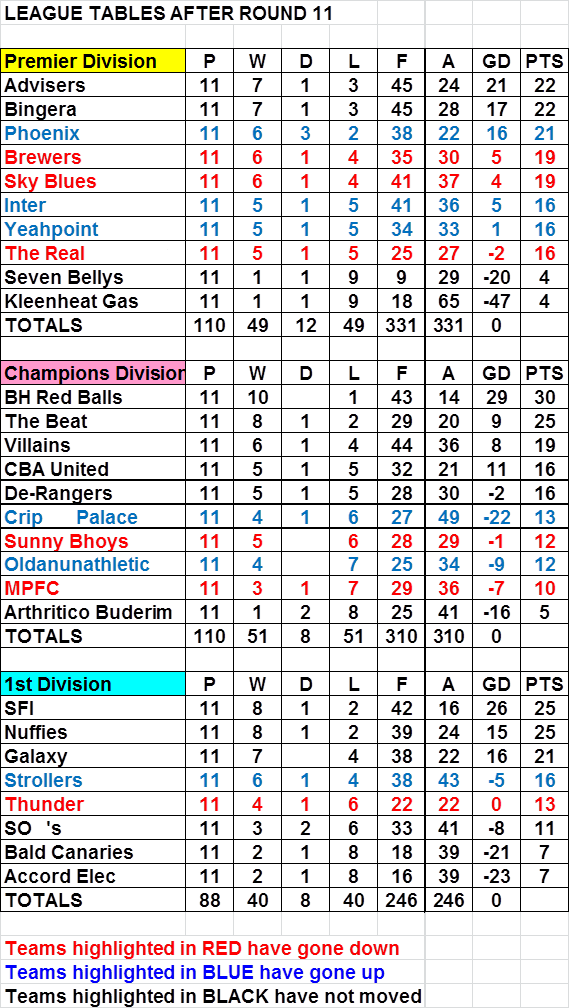
Every number in the league table above is hard keyed except for the 'Totals' rows! EVERY NUMBER.
Not only that, each week he had to manually rearrange the order of the teams as rankings changed, and update the colour coding for the teams that moved up or down.
No wonder it took 2 hours to update every week.
All that manual work is an Excel crime!
When we heard about this we thought it was a prime candidate for an ‘Excel Dashboard Extreme Makeover’.
So I put on my Dr Dashboard mask and nipped and tucked his league tables into shape.
And here is the ‘After’ photo:
Note: The after photo shows the current season’s teams and divisions which are slightly different to the before photo from last season, but I think you get the gist. It’s much better, right?
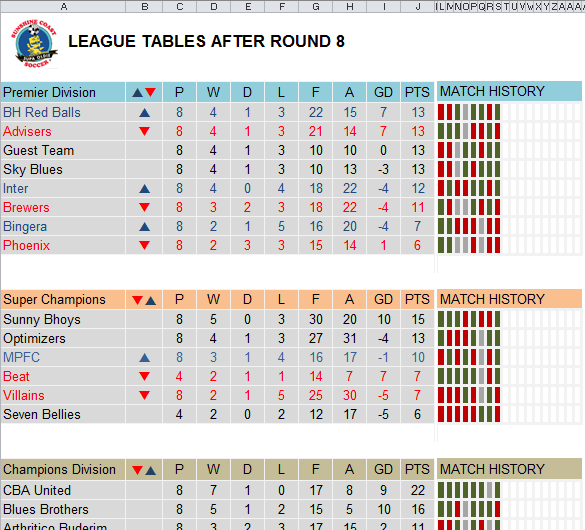
In complete contrast to the original league table every number is now the result of formulas that automatically recalculate. EVERY NUMBER.
Not only that, the teams are automatically sorted based on their new rankings and the colours and symbols also automatically change with the help of Conditional Formatting.
It now takes Darryl 10 minutes to update. In reality it could take 2 but he uses one finger to type.
It’s Excel heaven! Actually, it’s the way Excel was intended to be used.
Anatomy of the Dashboard
Hopefully you’re not squeamish because I’m going to take you into the gizzards (as my kids say) of this new league table dashboard so you can see how it works.
Note: Even if you're not interested in football, there are some great lessons here on different tools you can use in Excel and how to tie them together to make a dynamic and informative report.
So back away from the mouse and keep reading 🙂
Download
Download the workbook and follow along. Use it for your own league tables, reverse engineer it and see how it works, or print it off and make a paper plane, whatever tickles your fancy!
Enter your email address below to download the sample workbook.
Source Data
Like I said, previously all of the data was hard keyed except for the ‘Totals’ row which was only there for checking that he’d keyed everything in correctly. It was good to see that he'd built in cross checks.
With the new league table he simply enters the fixtures and scores for the week into a source data sheet for each division. The Premier division looks like this:
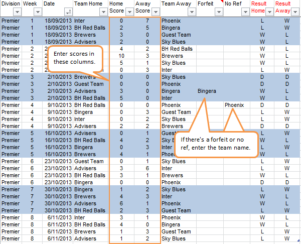
You might be thinking, phew that’s a lot to key in, but in reality he already has almost all of this data for the fixtures draw. Formulas in the Result Home and Result Away columns return the W, L or D (win, loss, draw), so nothing to enter there.
And in actual fact he can set everything up in advance then once a week he completes the Home and Away scores, and if there’s a forfeit or no ref he enters them. 10 minutes later it’s all done!
By the way, the W, L or D feeds the Match History conditional formatting in the league table. More on that in a moment.
Workings
The league tables are fed by two sets of workings in columns to the right; one for the current week (columns AG:AR) and one for the previous week (columns AT:BD partially outside of image):
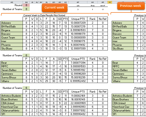
In columns AH to AM and AR I’ve used SUMPRODUCT formulas, but you could also use SUMIFS and COUNTIF(S) to return the results.
- P – Played SUMPRODUCT or COUNTIFS
- W – Won SUMPRODUCT or COUNTIFS
- D – Draw SUMPRODUCT or COUNTIFS
- L – Lost SUMPRODUCT or COUNTIFS
- F – Goals For SUMPRODUCT or SUMIFS
- A – Goals Against SUMPRODUCT or SUMIFS
- No Ref – SUMPRODUCT or COUNTIF
GD – Goal Difference is simply column AL – AM, and the PTS (Points) are referencing the values in cells AP2:AR2 located above the workings tables.
I’ve used the RANK function (column AQ) to rank the teams in the League Tables from top to bottom.
Note: because there could be ties I’ve first calculated a ‘Unique PTS’ in column AP which is weighted to avoid a tie on Points (PTS). It does this by also using the Goal Difference (GD) and an alphabetical ranking in the calculation.
The League Tables
The Rank result is then used in a VLOOKUP formula with CHOOSE to return a sorted list of teams in column A of the league table.
Tip: we use CHOOSE to get around the limitation of VLOOKUP not being able to lookup to the left. You could also use INDEX & MATCH.
Fonts and Conditional Formatting
Now, you might have wondered earlier why we need workings for the current week and previous week…well that’s because we need to show which teams have moved up, down or stayed the same from one week to the next.
I’ve done this with some wingding fonts in column B, and Conditional formatting is used to highlight the team’s row red if they moved down, blue if they moved up and black if they stayed the same.
Match History
The match history is also conditional formatting.
An INDEX and MATCH formula looks up the ‘Result’ columns on each division’s source data sheet and brings in the W (win), L (loss) or D (draw) for each week. Conditional formatting colours the cell green (W), red (L) or grey (D).
The challenge with this formula is that because the order of the teams shuffles each week the Match History also needs to shuffle to stay aligned to the team's new position in the league table.
Zebra Stripes
Did you notice the Conditional Formatting Zebra Stripes on the source data sheets?
The blue and white alternating lines allow you to easily see the records for each week's fixtures grouped together in banded blue/white lines.
You can learn how to do Zebra strips in varying numbers of rows here.
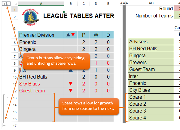
Group Buttons
I have used Group Buttons to hide the spare rows for each division. This allows the dashboard to be re-used from one season to the next and allow for changes in the number of teams.
I prefer to use Group Buttons to hide/unhide rows and columns as I find it quicker to toggle between them being hidden or unhidden.
More on how to group and outline data here.
Want More?
Do your reports take hours to update like Darryl's did?
If you'd like to learn how to create dynamic reports like this that take just a few minutes to update, then check out my Excel Dashboard course where I teach these techniques and more.
Thanks
Thanks to Roberto for helping me make my Match History formula more elegant.

I have watched your content on YouTube and you’re really amazing. Your dashboards are super neat, organized, and very clean. I admire that a lot.
Quick question though; how do you draw those little shapes in excel (the red signaling a decline in performance, and a green showing an improvement in performance)?
Hi Muchwa,
Thanks for your kind words 🙂
The red/green markers are done with Conditional Formatting (download the file and inspect how it’s done). You can also use Sparklines.
Mynda
Is there any way to update the match history to more than 18 rounds?
Sure, you just need to add more columns and copy the formulas across accordingly. You’ll also want to add to the data validation list in cell AI1.
Mynda
This is. Soo helpfull
Pity I won’t return as match secretary of our social league next year.. I will pass on the knowledge picked up here though!
Thank u
Glad you liked it, Sherman.
Mynda,
Thank you for this excellent dashboard. I’m in an old man softball league and have modified your sheet to help the league manager present the results each week. I am having a bit of difficulty because we rank differently.
The current sheet sorts based on wins(pts), then sorts on run differential. This would work in most leagues but, our second ranking is based on head to head results, then run differential.
I am at a loss of how to create a formula that evaluates any team with the same win/loss record based on head to head results.
Any ideas? Perhaps a manual sort would be the easiest in our situation. It has been a fun challenge for my excel skills however!
Thanks again.
Hi Brendon,
I’m not sure what you mean by ‘head to head results’ but if you can send me your workbook via the Help Desk with an explanation of what you want and how it should appear when sorted then I can take a look.
Kind regards,
Mynda
Hi Mynda,
Have played around with this to no avail…
Our League consists of 10/12 per division, however our top division is split into 2; Premier/Section One and both sets of teams play each other as if it was only one division but their results are displayed as separate divisions as shown below.
This is how the league table is split
Premier Section League Table 15/02/2015
Pos Team Pld W L D For Agn Pts
1st Abingdon Allstars 15 14 1 0 155 85 155
2nd Rileys Red Devils 14 9 5 0 114 18 114
3rd Oracle A 15 9 6 0 119 13 119
4th West Oxford Democrats 14 12 2 0 141 72 141
Section One League Table
Pos Team Pld W L D For Agn Pts
1st Rileys A 14 5 9 0 100 10 100
2nd Donnington Social Club ‘B’ 15 7 8 0 106 13 106
3rd Marlborough Club A 15 6 9 0 105 15 105
4th Rileys Team Merola 14 5 9 0 104 2 104
5th Midget ‘A’ 15 0 15 0 60 105 60
6th Abingdon RBL 14 8 6 0 45 2 45
7th Railway Inn 15 5 10 0 30 45 30
8th BYE 0 0 0 0 0 0 0
and this is how the fixture appear for the opening 3 weeks
wk
1 BYE Oracle A
1 Railway Inn 4 11 Abingdon Allstars
1 Abingdon RBL 4 11 Rileys Red Devils
1 Rileys Team Merola 5 10 West Oxford Democrats
1 Marlborough Club A 10 5 Rileys A
1 Midget ‘A’ 5 10 Donnington Social Club ‘B’
2 BYE Donnington Social Club ‘B’
2 Rileys A 12 3 Midget ‘A’
2 West Oxford Democrats 8 7 Marlborough Club A
2 Rileys Red Devils 8 7 Rileys Team Merola
2 Abingdon Allstars 10 5 Abingdon RBL
2 Oracle A 11 4 Railway Inn
3 Railway Inn BYE
3 Abingdon RBL 5 10 Oracle A
3 Rileys Team Merola 6 9 Abingdon Allstars
3 Marlborough Club A 10 5 Rileys Red Devils
3 Midget ‘A’ 1 14 West Oxford Democrats
3 Donnington SocClub ‘B’ 7 8 Rileys A
Hi Kevin,
Can you not just enter them as though they are two separate divisions since that’s how you want the league table results displayed?
The fact that both teams may appear in both fixtures doesn’t matter.
Mynda
Hi,
You’ve allowed the tables for up to 12 teams but if the play each other HOME and AWAY it will take 22 weeks to complete, but you’ve only allowed for 18 weeks. How do I increase the number of weeks.
Looks great..
Hi Kevin,
In column BG add more weeks then increase the Data Validation source for cell AH1 to pick up the extra weeks. You’ll also need to insert new rows for each division and copy down the formulas.
Be careful when you insert the rows that you don’t mess up the data validation list source in column BG.
Hope that helps.
Mynda
Hello,
Can you please
1) Cell B4.How did you get these two symbols side by side (pq)
2)Cell AH5.Can you pls explain the formula as I am getting difficulty interpreting/understanding this formula
3)Cell AH18,AH33,AH48.What are their utilities?
Thank you
Hi Dennis,
1. IN B4, the font is Wingdings, that’s why pq is seen as symbols, instead of text, try changing the font, you’ll see what i mean.
2. The SUMPRODUCT formula has multiple arguments, it will return the count of rows where all arguments are TRUE :
(ISNUMBER(premier[Home Score])
(premier[Week]<=$AH$1) (premier[Team Home]=Results!AG5) ISNUMBER(premier[Away Score]) (premier[Week]<=$AH$1) (premier[Team Away]=Results!AG5) It is similar to COUNTIFS formula, where you can add multiple ranges and criterias to count: for example, the last 2 conditions will have the following syntax in COUNTIFS formula: =COUNTIFS(premier[Week],$AH$1,premier[Team Away],Results!AG5) In SUMPRODUCT, the conditions are wrapped in paranthesis and multiplied, this is the only difference. 3. In Super Champions sheet, there are only 6 teams, that's why in cells you mentioned the value is 6. You may replace that static value with a dynamic formula: =COUNTA(super[Team Home]), that will autoadjust when you add teams to that table. As the Instructions says, if you read them, you will find this mention: "The Match History formulas allow for up to 18 rounds. There is enough space for 12 teams in each division. To hide/unhide the spare rows use the Group buttons to the left of the row numbers " Regards, Catalin
How do you populate the Fixtures, do you do this manually ?
Hi Kevin,
Yes, you have to type in the fixtures yourself.
Mynda
Hi Mynda,
No problem with fixtures as I’ve been able to add a TEAMS sheet and use LOOKUP on the divisional sheets to populate the fixtures automatically by adding another 2 columns into which I input the 1 vs 2, 3 vs 4 etc….
Only problem I have now is that the Group buttons to the left of the row numbers only switch between 8 and 12 (I have league of 10) even after changing the “Number of Teams” box in column AH on the Results sheet
Kevin
Hi Kevin,
The group buttons need to be changed using the Group tool on the Data tab of the ribbon. First remove the groups that are there and then reapply the. Here is a tutorial on Grouping rows and columns:
https://www.myonlinetraininghub.com/excel-2007-group-and-outline-data
Kind regards,
Mynda
Thanks for the reply Mynda, managed to work it out for myself for a change
Kevin
🙂 Well done!
I am American like some of the other submissions, but this is something that I definitely will ponder and dissect. Thank you for these morsels.
Dan
You’re welcome, Dan 🙂
I am glad to your post, really the dashboard is working Excellent.Basically the formula you put here is making a proper structure what actually I was need keep it up!
Thanks Bruce, glad you found it useful.
Thank you very much for sharing this wonderful spreadsheet with us, Mynda, it’s a piece of art, I am amazed of what you can do to squeeze the power of Excel to the next level! As Bryan said, it’s difficult for me to understand what the numbers mean because I am not a big fan of sports, although soccer is very popular in Paraguay, but I must recognize that you did an awesome job rearranging all the data, it looks so different and interactive now!
Thanks, Juan. I’m glad you like it. Please download the file (if you haven’t already) and play around with it to see how the formulas work.
Kind regards,
Mynda.
Wow, so many clever things going on here. I don’t fully appreciate what all the numbers mean (I’m not into sports, and I’m American, so even if I were I wouldn’t be into soccer!), but Excel is Excel so the formulas themselves (mostly) make sense. I’m going to have to hunker down and play with a few of them to figure out exactly how they work. I think my favorite part is the ability to re-rank every week. That is definitely a trick I’m going to have to put in my book.
Thanks, Bryan 🙂 Glad you liked my treasure trove of Excel tricks.