Multi-level Dependent Drop-down Lists

Creating multi-level dependent drop-down lists in Excel can significantly speed up data entry and reduce errors. Whether you're managing data for different countries and their regions or any other related lists, dependent drop-down lists allow for a streamlined process.

However, these multi-level dependent drop-down lists used to be laborious to set up and maintain. But now with the power of dynamic array formulas, Excel makes this task easier and more flexible than ever before.

In this post, we'll explore two methods to set up these dynamic drop-down lists, including a mind-blowing trick that you won't want to miss.

Multi-level Dependent Drop-down Lists Video

Get the Example File and Cheat Sheet

Understanding Multi-Level Dependent Drop-down Lists

Multi-level dependent drop-down lists are where the options in one list depend on the selection made in another. For example, if you select a country from one drop-down, the next drop-down list will show only the regions or states related to that country.

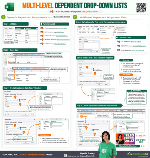
Method 1: Dynamic Dependent Drop-down Lists

This method leverages the UNIQUE, SORT, and FILTER functions to create a dynamic, spillable array that updates automatically as your data changes. It's great if you only have 2 levels.

Step 1: Set Up Your Data

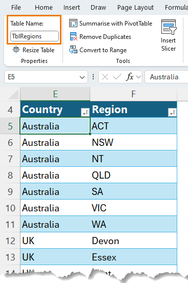
Begin with your drop-down list data structured in an Excel Table. This table should include columns for your main category (e.g., Country) which is level 1, and the dependent category (e.g., Region) which is level 2.

Step 2: Create a Unique List for Level 1

Use the UNIQUE function combined with SORT function and TRANSPOSE function to extract a list of your level 1 values, in my case it's countries, that dynamically updates. Here's the formula:

=TRANSPOSE( SORT( UNIQUE(TblRegions[Country]) ) )

You can see it spills the results across the row:

Step 3: Extract the Regions Based on Selected Country

Use the FILTER function to create a dynamic list of regions for each country:

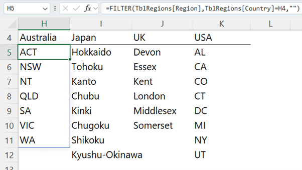
Cell H5:

 =SORT(FILTER(TblRegions[Region], TblRegions[Country]=H4, ""))

This formula filters the regions corresponding to the country in row 4:

Copy the formula across as many columns as required to allow for growth in the number of countries you might add to the table.

Tip: do not left click and drag to copy this formula. You must copy and paste to prevent the table references from changing.

Step 4: Set Up Data Validation

Select the cells where you want the drop-down list to appear, go to the Data tab > Data Validation.

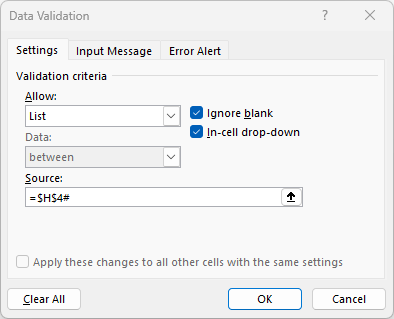
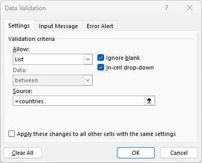
Set the validation criteria to allow a list, and reference the spilled array created by your UNIQUE function for countries:

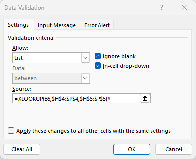
And for the region drop-downs again, select the cells you want the drop-downs, then Data tab > Data Validation:

 =XLOOKUP(B5, $H$4:$P$4, $H$5:$P$5) 

Limitations of Method 1:

This approach requires you to anticipate the maximum number of countries you might add, which can be cumbersome if your data grows significantly.

It also doesn't allow for you to add another level of dependency, like cities.

Method 2: Multi-level Dependent Drop-down Lists

This advanced method uses the CELL function to automatically detect the last edited cell, making the setup more flexible and scalable, especially if you have multiple levels of dependent drop-down lists.

Thank you and shout out to Peter Bartholomew for sharing this technique with me.

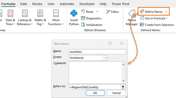
Step 1: Define Name for First Level

Define a name for the first drop-down list (level 1). In this example it's my country column in the table (e.g., "countries";).

Step 2: Set Up the Country Drop-Down List

In your data validation setup (Data tab > Data Validation), reference the named range for the country list:

This defined name will automatically include new items in the table, even if it's on another sheet.

Step 3: Create a Dependent Drop-Down List for Regions

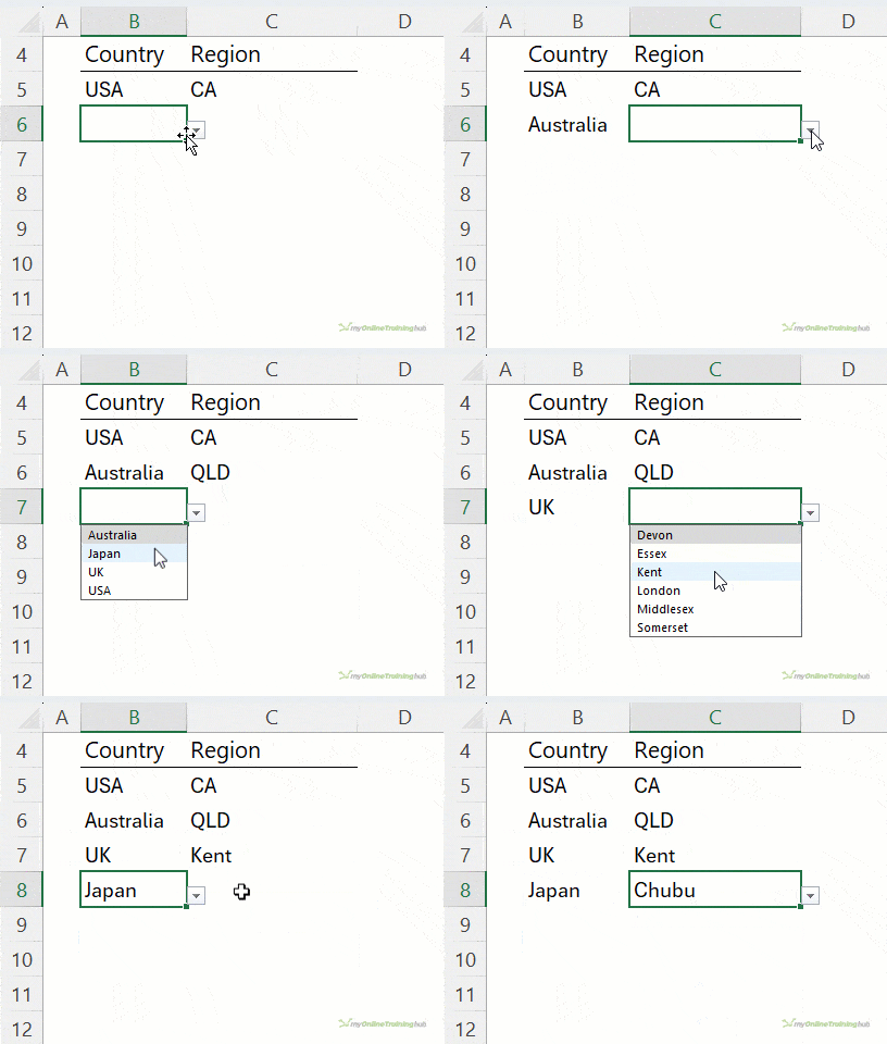
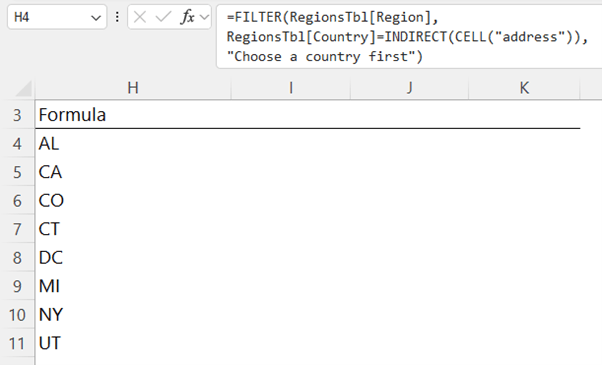
Use the CELL function to dynamically track the last edited cell and use the INDIRECT function to reference it in your FILTER function (see video for demonstration):

 =FILTER(RegionsTbl[Region], RegionsTbl[Country]=INDIRECT(CELL("address")), "Choose a Country First")

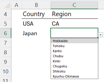
This setup allows the drop-down list for regions to update based on the country selected, without needing to predefine the number of countries.

Step 4: Trigger the Dependent Drop-Down

Ensure that the CELL function triggers correctly by editing the country cell, which will automatically refresh the dependent drop-down list for regions.

Adding More Levels and Handling Changes

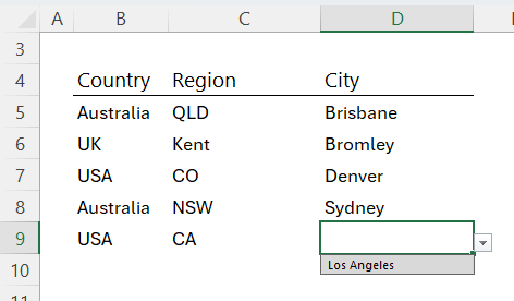
This method also allows for adding more levels, such as cities:

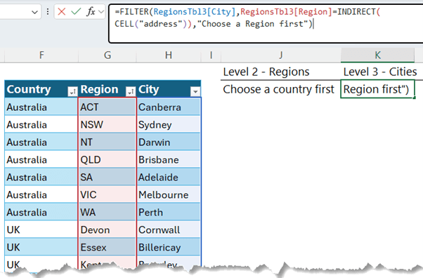
By simply modifying the existing formula to reference the next dependent list:

Important Note: The formula relies on the last edited cell being the previous drop-down list. If you need to edit a previous selection, make sure to re-edit the earlier drop-down list to ensure the dependent lists update correctly.

Method 2 Variation: Double-Click Drop-downs

If you want more flexibility, such as editing a previously selected drop-down list, you can use the double-click method.

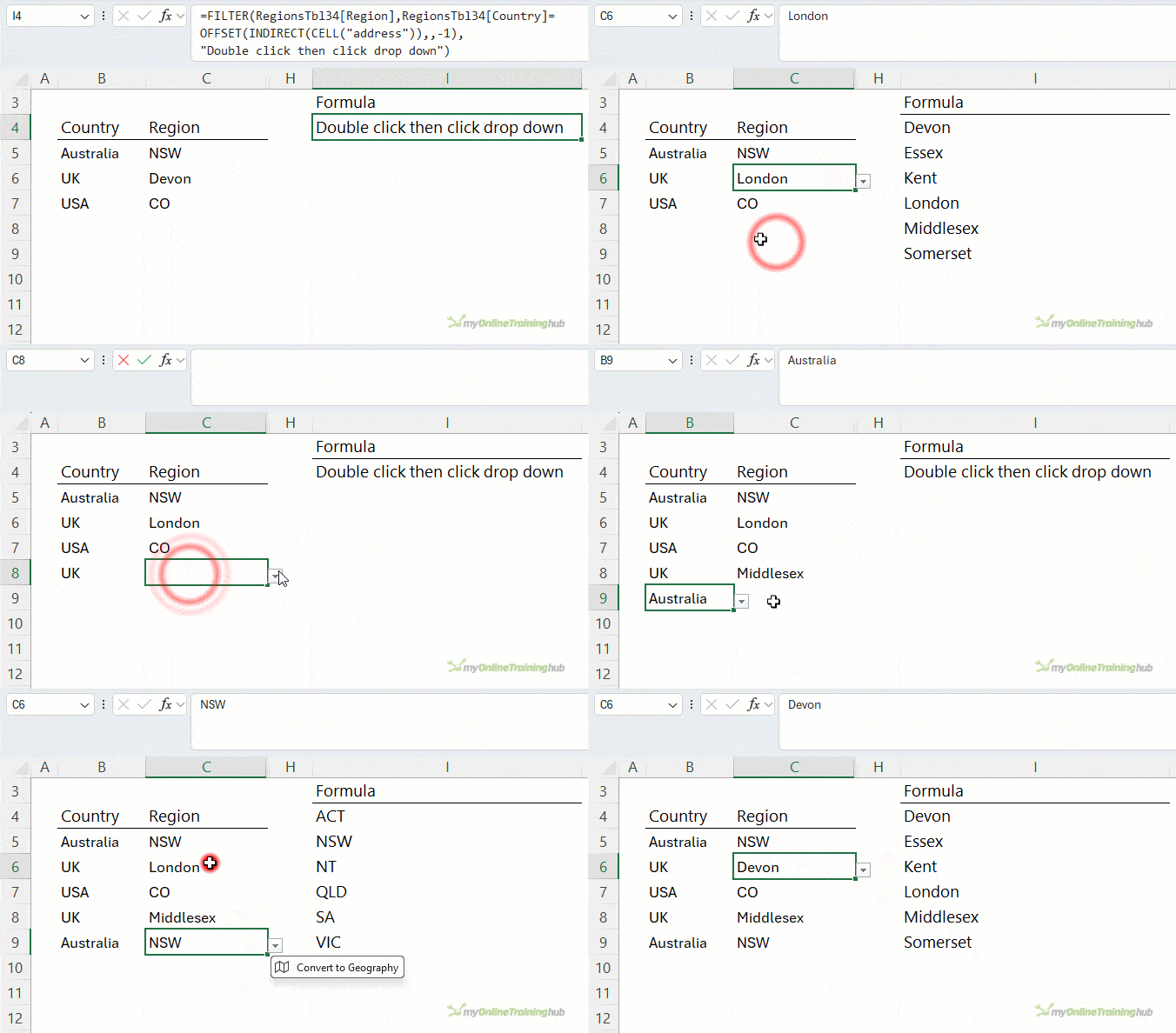
Double-Click the cell containing the drop-down you want to modify > select the new option from the drop-down list:

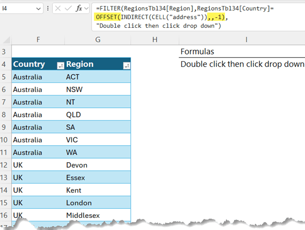
To accommodate this, use the OFFSET function to return a reference to the cell that is one cell to the left of the last edited cell.

Limitation: This method may not be intuitive to users, but once you demonstrate, they should be comfortable using it.

Next Steps

While both methods provide dynamic solutions for multi-level dependent drop-down lists in Excel, the second method with the CELL function offers more flexibility, especially when dealing with large datasets or multiple levels of dependency.

The use of the CELL function, in particular, is a game-changer, allowing for a more seamless and scalable setup.

If you're ready to dive deeper into the capabilities of Excel's dynamic array functions, be sure to explore our detailed guide on the FILTER function. Happy Excel-ing!