A while back Vernon asked me how he could search one cell and compare it to a list of words. If any of the words in the list existed then return the matching word.
Ugh, I’ve written that 3 times and I’m not sure it’s any clearer…let’s look at an example.
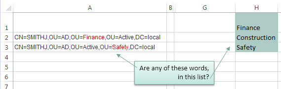
I’ve highlighted the matching words in column A red.
What we want Excel to do is to check the text string in column A to see if any of the words in our list in H1:H3 are present, if they are then return the matching word. Note: I’ve given cells H1:H3 the named range ‘list’.
There are a few ways we can tackle this so let’s take a look at our options.
Warning: this is quite an advanced topic which requires an array formula to solve it.
Update: It's easier and more robust to use Power Query to search for text strings, including case and non-case sensitive searches.
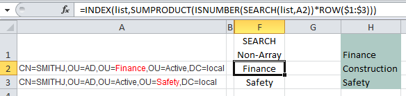
Non-Case Sensitive Matching
If you aren’t worried about case sensitive matches then you can use the SEARCH function with INDEX, SUMPRODUCT and ISNUMBER like this:
=INDEX(list,SUMPRODUCT(ISNUMBER(SEARCH(list,A2))*ROW($1:$3)))
In English our formula reads:
SEARCH cell A2 to see if it contains any words listed in cells H1:H3 (i.e. the named range ‘list’) and return the number of the character in cell A2 where the word starts. Our formula becomes:
=INDEX(list,SUMPRODUCT(ISNUMBER({20;#VALUE!;#VALUE!})*ROW($1:$3)))
i.e. in cell A2 the ‘F’ in the word ‘Finance’ starts in position 20.
Now using ISNUMBER test to see if the SEARCH formula returns any numbers (if it does it means there is a match). ISNUMBER will return TRUE if there is a number and FALSE if not (this gives us a list of Boolean TRUE or FALSE values). Our formula becomes:
=INDEX(list,SUMPRODUCT({TRUE;FALSE;FALSE}*ROW($1:$3)))
Use the ROW function to return an array of numbers {1;2;3} (see notes below on why I've used ROW in this formula). Our formula becomes:
=INDEX(list,SUMPRODUCT({TRUE;FALSE;FALSE}*{1;2;3}))
When you multiply Boolean TRUE/FALSE values they become their numeric equivalents i.e. TRUE = 1 and FALSE = 0. So our formula evaluates this ({TRUE;FALSE;FALSE}*{1;2;3}) like so: {1*1, 0*2, 0*3} and our formula becomes:
=INDEX(list,SUMPRODUCT({1;0;0}))
SUMPRODUCT simply sums the values {1+0+0} which gives us 1. Note: by using SUMPRODUCT we are avoiding the need for an array formula that requires CTRL+SHIFT+ENTER. Our formula becomes:
=INDEX(list,1)
Index can now go ahead and return the 1st value in the range of cells H1:H3 which is ‘Finance’.
Note: the above formula will not work if a match isn't found. If you want to return an error if a match isn't found then you can use this variation:
=INDEX(list,IF(SUMPRODUCT(--ISNUMBER(SEARCH(list,A2)))<>0,SUMPRODUCT(ISNUMBER(SEARCH(list,A2))*ROW($1:$3)),NA()))
Not as elegant, is it? In which case you might prefer one of the array formulas below.
Notes about the ROW Function:
The ROW function simply returns the row number of a reference. e.g. ROW(A2) would return 2. When used in an array formula it will return an array of numbers. e.g. ROW(A2:A4) will return {2;3;4}. We can also give just the row reference(s) to the ROW function like so ROW(2:4).
In this formula we have used ROW to simply return an array of values {1;2;3} that represent the items in our 'list' i.e. Finance is 1, Construction is 2 and Safety is 3. Alternatively we could have typed {1;2;3} direct in our formula, or even referenced the named range like this ROW(list).
So you see using the ROW function is just a quick and clever way to generate an array of numbers.
What you must bear in mind when using the ROW function for this purpose is that we need a list of numbers from 1 to 3 because there are 3 words in our list and we’re trying to find the position of the matching word.
In this example the formula; ROW(list) will also work because our list happens to start on row 1 but if we were to start 'list' on row 2 we would come unstuck because ROW(list) would return {2;3;4} i.e. 'list' would actually reference cells H2:H4.
So, don’t get confused into thinking the ROW part of the formula is simply referencing the list or range of cells where the list is, the important point is that the ROW formula returns an array of numbers and we're using those numbers to represent the number of rows in the 'list' which must always start with 1.
Functions Used
ROW - Explained above.
Case Sensitive Matching
[updated Dec 5, 2013]
If your search is case sensitive then you not only need to replace SEARCH with FIND, but you also need to introduce an IF formula like so:
=INDEX(list,IF(SUMPRODUCT(ISNUMBER(FIND(list,A2))*ROW($1:$3))<>0,SUMPRODUCT(ISNUMBER(FIND(list,A2))*ROW($1:$3)),NA()))
Unfortunately it's not as simple or elegant as the first non-case sensitive search. Instead the array formulas below are nicer
Array Formula Options
Below are some array formula options to achieve the same result. They use LARGE instead of SUMPRODUCT, and as a result you need to enter these by pressing CTRL+SHIFT+ENTER.
Non-case Sensitive:
[updated Dec 5, 2013]
=INDEX(list,LARGE(IF(ISNUMBER(SEARCH(list,A2)),ROW($1:$3)),1)) Press CTRL+SHIFT+ENTER
Case sensitive:
[updated Dec 5, 2013]
=INDEX(list,LARGE(IF(ISNUMBER(FIND(list,A2)),ROW($1:$3)),1)) Press CTRL+SHIFT+ENTER
Download
Enter your email address below to download the sample workbook.
Thanks
Special thanks to Roberto for suggesting the 'updated' formulas above.

Thank you for this post, exactly what i am searching for!
What if there are multiple matches in A2 from the list in H columns. I think it should work fine right :)?
Great to hear, Srikanth. If you get stuck with the multiple matches scenario, please post your question on our Excel forum where you can also upload a sample file and we can help you further.
Thank you i have made the post as asked 🙂
Hello,
Using “=INDEX(list,LARGE(IF(ISNUMBER(SEARCH(list,A2)),ROW($1:$3)),1)) Press CTRL+SHIFT+ENTER” and it returns “0”. How to fix it? it used to work for me. Thank you in advance for your help!
Bing
Hi Bing,
Please upload a sample file on our forum (Create a new topic) so we can see what’s wrong, the error might not be in the formula.
Thank you very much Catalin! It’s resolved now. It was caused by an empty cell in the end of the name list. Thanks again!
Bing
Hi
Is possible to sum all WA11?
(A1) WA11 4
(A2) AdBlue 1, WA11 223
(A3) AdBlue 3, WA11 32, shift 4
… and everything is in one column.
Thanks you very much for your help.
Sincerely Marko
Hi Marko, it’s difficult to visualise the structure of your data. Please post your question on our Excel forum where you can also upload a sample file and we can help you further.
Hi Mynda,
Thanks for the useful videos and tips.
An alternative is to use SEQUENCE(3) instead ROW($1:$3) for the above example.
Use of the ROWS function inside SEQUENCE (e.g. SEQUENCE(ROWS(named_range)) allows the size of the sequence to be of variable length (if desired.
This would eliminate use of the volatile function INDIRECT which may increase calculation time.
You may already be aware of this technique, but I think the above page could be improved with a change away from the ROW technique
Yes, now that we have dynamic array functions, like SEQUENCE, there are far better ways to achieve this. Of course only a small portion of Excel users have access to dynamic arrays, so for now the above technique is still relevant. Thanks for sharing.
Hello,
I want to search a all the related records of a value that is in cell D2
from a list of thousand of rows in column A.
The value can occur multiple times with multiple items.
For example, an item# 123456 in cell D2 may have multiple records and can be placed anywhere in text string of the rows in column A such as
123456_shirt
123456_boots
tie_123456
Suit_123456_black
Watch_123456
I want a formula that can search the Value of cell D2 in all the rows of column A and put all the values it finds (full string name) one by one in column E2, E3,E4, so on
In simple words, if we click on “find button” in excel and give it a value to find, it shows all the related match values available anywhere in the database. Then we can navigate by clicking next button.
I want to do it using a formula, because I have a list of values to search and cant search one by one manually.
Is there any way to do it?
Hi Sunil,
You haven’t said which version of Excel you have, so assuming you have Microsoft 365, you can use the FILTER function, where your list is in cells A2:A6:
If you don’t have Microsoft 365, please post your question on our Excel forum where you can also upload a sample file and we can help you further.
Mynda
Thank you for this article. With regards to the formula without case match (the first formula), I noticed that for the following 2 cases, it does not work:
Case 1:
Value in A1 is:
What is the Total of Finance, construction?
In this case it returns Safety.
Case 2:
Value in A1 is:
What is the Total of Finance, construction and safety is?
In this case it returns #REF!
I am using Excel 2007.
Your help is appreciated.
Thank you much.
Hi Emmad,
Please upload a sample file where we can see your attempts, important information is not provided. Use our forum for upload, create a new topic after sign in.
Great formula! Here’s an embellishment – use the INDIRECT and ROWS function in calculating the number of rows in the list range:
=INDEX(list,IF(SUMPRODUCT(–ISNUMBER(SEARCH(list,A2)))0,SUMPRODUCT(ISNUMBER(SEARCH(list,A2))**ROW(INDIRECT(“$1:$”&ROWS(list)))),NA()))
This means that if you change number of item in the the list then you do not need to update the formula each time this happens.
Thanks for sharing, John.
Hi,
I’m also having trouble with SEARCH( Named_Range, A2) not working I have text in the named list (located on same worksheet) which does exist in cell A2, but the search formula does not return any value. The SEARCH function does work however when I limit the range to one cell. Any suggestions?
Jay
Hi Jay,
If your list has more than 1 cell, we are talking of an array of results, so it is an array formula that will return a list of matches: {#VALUE!;20;#VALUE!;#VALUE!}, as explained in the article. Are you using the SEARCH function alone?
I think the question will be
What if the list of matches return : {#VALUE!;20;#VALUE!;40}.
We will have two matching words in the row. How can we do index search of two values?
Hi Will,
Please post your question on our Excel forum where you can also upload a sample file that illustrates your scenario and we can help you further.
Mynda
this fomular always show the first word in the list
Hi Dunget,
Have you tried the workbook provided?
Or you tried to apply this on your own version? If this is the case, you should double check your formula, because works on the sample book.
You can upload your version on our forum so we can see what’s wrong.
IS there any way where the formula can refer to the rows of different worksheet or workbook?
Because my data starts from row 3 but the criteria range is placed in different workbook, it works till there but when it comes to the ending part, the row reference is of the lookup sheet only.
I have tried referencing rows from my another worksheet but and it gives a #N/A error.
Any help would be appreciated.
Hi Rishabh,
Not sure why you are trying to reference rows from another sheet. You can have the criteria list in another sheet, the formula will still work. The only thing you need to adjust is the ROW($1:$3) part, to match the exact number of rows in the criteria list. It does not matter to what sheet ROW($1:$4) is coming from, as it’s just a way to return a list of numbers from 1 to 3 (or to the max number of rows in the list).
There is one scenario where the formula does not work: if there are multiple matches.
In this case, you should add a MAX or MIN function, to return the first or the last match only:
=INDEX(list,SUMPRODUCT(MIN(ISNUMBER(SEARCH(list,A2))*ROW($1:$4))))
MIN function in these cases will count 0s since it is the minimum value and hence will evaluate to #N/A even when multiple matches are found. I think using SMALL solves that. Please suggest.
Hi Praveen,
The formula works as described, I suggest you should test it.
In the file provided for download, there is another version using LARGE, use any flavor you like.
Cheers,
Catalin
Hi all,
I am new here and dont know how this question in the comments work. Please guide.
My question here is, for the same data, if the situation above is vice-versa. What would be the formula. If i have to identify H column words from the rows 1 to 5. How would i do that.
Thank you
Hi Ismail,
Please upload a sample file on our forum, it will be easier to understand your situation and help you. (create a new topic after sign-up)
Sure. Thaank you. I will post it in forum.
Any help. I am desperately waiting..
SEARCH( Named_Range, A2) does not work ! I have text in the named list (located on a different worksheet) which does exist in cell A2, but the search formula does not return any value, therefore the rest of the formula does not produce the desired result.
Hi James,
What text you have in cell A2 and what text you have in that NamedRange that contains the A2 value?
If you have “finance manager” for example in A2, and in the NamedRange you have only “finance” or just “manager”, because A2 text should be completely included into NamedRange values.
I am new to excel formulas and such, and I am really struggling with this. I downloaded the example, but I still am not getting the results I want.
Using your example, I moved my data to A and B columns (3500 rows). I have a list keywords in column H (named list and contains1500 words) which I would like to find just in B column, and just mark Column C with True or False.
I used Search Non-Array: =@INDEX(list,SUMPRODUCT(ISNUMBER(SEARCH(list,B3))*ROW($1:$1500)))
And all I get is #N/A. What am I missing?
Hi Pat,
That formula won’t evaluate to TRUE or FALSE, but there is another problem that needs fixing first if it’s returning the #N/A error. Can you please post your question on our Excel forum where you can upload your Excel file so we can take a look at what is causing the error?
Mynda
Would this work for emails? I’m getting some data via a Google form. I’d like for it to check the column for a specific email. If that email is not on the list, I’d like for it to show the email. Then, I won’t have to email an entire group contact to fill out the form. I’d like to only email those folks whose emails do not show up in the column.
Possibly Mark, hard to say without seeing your data and fully understanding what you are trying to do.
Can you start a topic on the forum and include your workbook.
Regards
Phil
I am currently trying to use this but not returning results. I’ve matched the formula and tried other iterations but no luck with returned values.
Hi Garrett,
Hard to say what is happening without seeing what you’ve done.
Please post a qs on the forum and include your workbook.
Regards
Phil
Hi. What if more than one value from the list is found in a single cell? It is returning the #NUM! error. I would like to return the first value found in the text string. Thanks
Hi Pedro,
Please use the formula at the end of this post, changing ‘LARGE’ to SMALL e.g:
=INDEX(list,SMALL(IF(ISNUMBER(SEARCH(list,A1)),ROW($1:$2)),1))
This will return only the first keyword found.
Mynda
Hi there,
Is there a wall to insted of returning a single value, returning all values in a concated format?
It is possible, but with newer excel versions that support the TEXTJOIN function;
=TEXTJOIN(“;”,TRUE,INDEX(list,IF(ISNUMBER(SEARCH(list,A2)),ROW($1:$3),0)))
Note: in the list, the first value should be empty always!
This was very helpful!
I needed to create a flag if any specific names were contained in fields (sometimes where multiple names were included). I couldn’t get the INDEX function to work properly, but the SUMPRODUCT combined with SEARCH did the trick.
Great work, Mynda!
Glad it was of use to you, Jonathan 🙂
Very useful. If there are multiple matches, can excel return these matches into multiple cells?
Hi Emily,
Yes, it is possible, see this article.
Could you elaborate, how exactly this would work?
thanks
Select a range of cells, put this formula in formula bar, and press ctrl+shift+enter, as described in the article provided: https://www.myonlinetraininghub.com/excel-multi-cell-array-formulas
=INDEX(list,IF(ISNUMBER(SEARCH(list,A2)),ROW($1:$3)))
Brilliant!
I needed this as part of a worksheet that will replace the download and classify functionality that Quicken has removed from its latest version (unless you pay a monthly fee). I need to parse CSV files I download from my bank and credit card company, standardizing the downloaded names, adding categories, and then converting from row-column to the simple Quicken “QIF” format.
I know you did created these formulas a long time ago, but your work is still helping people.
Thanks!!!
BTW, your true array formula is far more robust and deals with situations such as having a cell which contains TWO of the words from the list. It is also more forgiving if the ROW function is fed a number of rows that doesn’t match exactly the number of rows in the “list”.
Thanks for your kind words, John. Glad we could help 🙂
Perfect Catalin!
Thank you!
You’re welcome 🙂
This formula was truly a blessing for my needs. Thank you!
I have a small issue that perhaps cannot be corrected, but I am hoping there is a way. I tried some alternatives listed in the replies and they did not achieve the desired results either.
My list is a list of employees. The problem happens with Jenn and Jennifer. The result is always “Jenn”, regardless of whether the text is Jenn or Jennifer. My workaround was to do a search and replace of Jennifer = Jenifer.
Is there a way to force case-insensitive exact match?
Hi Michael,
Depending on how the text looks in the cell, you should change the Jenn entry from the list of employees to: “Jenn ” (with a space after, instead of space you can use any delimiter you actually have in that text)
Hi! How would you expand this formula if there were multiple matches in the list.
Let’s say there are several matches from the list of values and I want to produce a concatenated list of these found list values in the new cell.
Example, in A2 we find a match for Finance, Construction, Safety and we want to new cell to contain “Finance; Construction; Safety”.
Thanks!
Sami
Hi Sami,
Only a custom vba funcion can do that, excel functions cannot join arrays of matches.
You might use the new array functions, but Dynamic Arrays are only available in Office 365 for the moment.
I created a formula that will concatenate 2 matches:
=INDEX(Types1A, SMALL(IF(ISNUMBER(SEARCH(Types1A,B17)), ROW(INDIRECT(“$AN$1:$AN$”&COUNTA(Types1A)))), 1)) & IF(SMALL(IF(ISNUMBER(SEARCH(Types1A,B17)), ROW(INDIRECT(“$AN$1:$AN$” & COUNTA(Types1A)))), 1) = LARGE(IF(ISNUMBER(SEARCH(Types1A, B17)), ROW(INDIRECT(“$AN$1:$AN$” & COUNTA(Types1A)))), 1), “”, ” ” & INDEX(Types1A, LARGE(IF(ISNUMBER(SEARCH(Types1A, B17)), ROW(INDIRECT(“$AN$1:$AN$”&COUNTA(Types1A)))), 1)))
Press CTRL+SHIFT+ENTER
It’s basically Catalin’s formula twice (once with LARGE and once with SMALL) and an IF statement to concatenate if they are different values.
Great Formula, Catalin! Super Helpful
When I do =search(list,A2) I get a VALUE error with or without ctr + shift + enter and I’m going to blow my brains out
Hi Nick,
Please post your question and Excel file on our Excel forum where we can help you further before something bad happens 😉
Mynda
I am having a problem with the formula. Whenever it doesn’t find a match in the phrase, it returns a value from the list. I expected to get an error message instead. Any suggestions on how I can fix this issue.
Hi Rafael,
If you download the workbook you’ll see the formulas in columns E, J and L all return errors if a match isn’t found. Try using one of these instead.
Mynda
Hi there, this is great and actually returns what I wanted (well kind of) but it’s doing something weird which i need help with!
So I wanted the formula to look in a cell of text containing a country name, find it based on matching it to a list of countries, then return that country name. Basically extracting the country name from the text so I can use it for other formulas.
I’ve done the above formula using a list called “COUNTRY” which has all the possible country names in, and it has returned a country name. BUT it’s returning the country which is 3 rows down from the country it’s supposed to be showing, for example the country listed in a cell is “Iceland” and it’s returning “Iran”. I’ve dragged the formula down to other cells and it’s doing the same thing, United Kingdom is pulling through Uruguay. Very weird! if you could shed some light as to why it might be doing this that would be fab, I assume it’s to do with the “ROW” numbers i’m putting in……
thank you!
Chloe
Hi Chloe,
Can you please upload a sample file on our forum? Without seeing what you have, I cannot tell you why you got that result, the answer is in your data.
Here is a link to our forum, just create a new topic after sign-up.
Catalin
Hi Catalin,
Thank you so much for coming back to me, I managed to crack it after taking a break from it! It was because my rows didn’t start at “1”. I realise that you’ve said in response to someone else that as long as the named list points to the same cells that shouldn’t matter but that didn’t seem to work for me. So I just moved the named list to start at row 1 instead of row 4 and it worked. If i have any further questions I’ll add them to the forum as you’ve suggested.
Thanks again!
Chlo
Hi
I modified this for use in a table:
=INDEX(Investment_Name,SUMPRODUCT(ISNUMBER(SEARCH(Investment_Name,[@Narrative]))*ROW(INDIRECT(Row_Range))))
Investment_Name is the list to be compared.
[@Narrative] = is the text containing the Investment Name
Row_Range = =”$1:$”&InvestmentNameCount
Many thanks for the formula!
You’re welcome, Philip. Thanks for sharing your version of the formula.
Mynda
Is any way (without VBA) we can return two matching words instead of just one in above example?
I mean if word “construction” and “safety” both are existing in Cell A3, can BOTH words found and able to display in Cell F3.
Many Thanks
Owen
Hi Owen,
In the downloadable workbook, select range L2:N2, type in the formula bar this formula:
=INDEX(list,LARGE(IF(ISNUMBER(SEARCH(list,A2)),ROW($1:$3)),COLUMN($1:$3)))
Then press Ctrl+Shift+Enter.
In H2, type “Active”, to test the formula.
This will give you an array of results.
There is no way without vba to return an array of results into a single cell, excel by default will return an array of results into an array of cells only.
Cheers,
Catalin
Hi Catalin,
I tried this and it works but only if I select a larger range. If I select just L2:N2 it doesn’t work but if I select L2:N3 it will. Any advice so it just appears horizontally?
Thanks
Hi Emily,
Have to see your data file, can you upload a sample on our forum so I can see what you did?
Hello,
I’m trying to use this formula to extract cities names within a string using a separate list of cities but I found it is not sensitive enough to get the exact city name. For example, I have the following address in E2:
Department of Life Sciences, MRC Centre for Molecular Bacteriology and Infection, Imperial College London, London SW7 2AZ, United Kingdom
Let’s say I have a list of all the cities in the uk (list name: “UK”) and I’m comparing that list against the list of addresses I have, one by one. How could I extract the correct city name?
The format of the addresses I have are not standardized, so the cities may end up in different positions with the string and also may or may not have delimiters between the city names.
Hi Antonio,
Please post your question and sample Excel file with the scenarios you’re referring to on our Excel Forum so we can see your question in context and help you further.
Mynda
Kinda lost here. I have a situation where I expect multiple matches (up to 20) and I want to output all of them. Is there anyway how I can return each value one by one?
Hi Johannes,
It’s difficult to say without seeing your scenario in an Excel file. Can you please post your question and sample file on our Excel Forum where we can give you a specific solution.
Thanks,
Mynda
hi Mynda
This scenario solution as exactly what I was looking for except it only works in your test situation and not in my spreadsheet. I downloaded your sample file and modified it and that also started giving incorrect results. This is what I did with your file.
* I added more terms to your list (col H) so it went down another 8 rows.
* I edited the name list so it went from row 2 to row 12
* I edited your formulas so the “ROW($1:$3)” became “ROW($1:$11)”
Hit F9 for refresh
in the first 2 formula columns I got #N/A now
in the last 2 formula columns I got a results but they chose options from my list that were incorrect.
If i just left the list from rows 1:3 and changed names in the list or modified the string in column A, the formulas worked fine, but when I added more items to the list and changed the named named range it would go screwy. such a shame as it exactly what I am looking for except in my situation the lookup named range is 120 rows.
Hi Scott,
Happy to troubleshoot further for you if you can post your question and Excel file in our forum here: https://www.myonlinetraininghub.com/excel-forum
Cheers,
Mynda
Hi Mynda,
I’m having the exact same issue as the commenter above. Were you able to find a solution for this problem? I tried searching the linked forum but could not find the conversation linked to this comment.
Hi Jack,
I can’t replicate the issue Scott had. Please post your question on our Excel forum where you can also upload a sample file and we can help you further.
Mynda
Hi I’m looking for a vba solution for the following:
Sheet1 Col A: Group Name
Col B: list of comma separated terms (for this Group)
Sheet2 Col A: text string
Col B: Group Name
I need to loop thru all the Groups in Sheet 1 and check if any of the terms in Sheet1 ColB appear in the text in Sheet2 Col A, if a match is found then copy the Group Name (Sheet1 ColA) to Sheet2 ColB and continue with the next cell in Sheet2 Col A.
What I have so far is:
For each cell in Sheet2 Col A
For each Group in Sheet1 Col A
If a word in Sheet2ColA is found in Sheet1 ColB then
Copy Sheet1ColA (Group Name) to Sheet2 ColB
Exit For
End If
Next Group
Next cell in Sheet2 ColA
Need help to write the VBA
Thanks
David
Hi David,
Please prepare and upload a sample file on our forum, it will be easier to work with a sample of real data.
Catalin
Hi Catalin, I found a solution, I’ll try and load it to the forum.
Thanks
David
Hi David,
Thanks for feedback. If you need more help, we’ll continue on forum.
Cheers,
Catalin
This is a fantastic solution, it works perfectly for me when expanding the index array to two columns and returning the second column as a “lookup” value from the list. Thank you!
Glad to see you’re happy Dave, thanks for the kind words 🙂
Thank you for your help 🙂 One build I made… I had a scenario where two matches were made from my list – for example, row 1 and row 4 of my list of search criteria were matched, and therefore the SUMPRODUCT returned ‘5’, so I replaced the SUMPRODUCT with a MAX to return the forth item as this suited what I needed.
Thanks for feedback Dave, indeed there are cases when multiple matches can be found.
My list doesn’t start in row one, what would be the alternate of my list doesn’t start in row one?
Thank you
Hi Jappie,
You just need to make sure the named range ‘list’ points to the cells containing your list.
And if your list contains more than 3 rows then you change the ROW formula to suit. e.g. if your list is 5 rows high then the ROW part of the formula will be ROW(1:5)
If you get stuck please post your question on our Excel forum with your sample Excel file so we can help further.
Mynda
I thought this was extremely helpful, until I hit a problem.
I have a list of cities, however some cities appear twice, with the second city an abbreviated version of the first.
For instance in cells H1 and H2…
CHICAGO
CHIC
The formula will work for CHIC, but not CHICAGO.
In A2 and A3…
CHICAGOMPREMIX-11310717-b
CHICFIELD—61290717
Is there any way around this???
Hi Kirsty,
You forgot to mention which formula are you using.
The SUMPRODUCT version has a downside: if more than a keyword is found, SUMPRODUCT will return the sum of their row positions, which will be wrong. Use the formulas from the end of the article:
=INDEX(list,SMALL(IF(ISNUMBER(SEARCH(list,A1)),ROW($1:$2)),1))
This will return only the first keyword found.
Catalin
Hi, Catalin, your formula works for me but it’s giving me an error when the list have blanks. Do you have a formula that can fix that?
Thanks!
Hi Ralph,
Keep the list without blanks, that’s the best option. Otherwise you will have to build another list from this list, without blanks.
HI Mynda, Please help me with this:
I need search-find numbers in a cell values is separated by comma, like this 8068,8069,8208,8713 | 7851,7859 | 7851,8208,8252 | 7738 | on this file ISNUMBER() is FALSE, “numbers” is on ROW ($1:$4) (file with 1500 rows), I not want split column, just want back TRUE or FALSE, in case of number is in cell separated by comma, or back number of ROW.
Thanks for ALL your Blogs and Tricks send by email.
Hi Carlos,
Can you please post your question and a sample file on our Excel Forum. I’m having trouble visualising your data structure.
Thanks,
Mynda
Thanks for a well worked / explained approach, was able to use with my data extremely easily. Appreciate it.
Cheers Phil
You’re welcome.
I changed the very first formula to: =INDEX(list,SUMPRODUCT(ISNUMBER(SEARCH(list,H2))*ROW(list))) since my data was in H2 versus A2. When I enter this formula and drag it down, it simply pulls the key words in order instead of returning the keyword if found in the H row cells.
Document Header Text Found Keyword
RRC PMO Accr AAA
Move Indy Dec Acquisition
Jan 2016 RRMC Rent Admirals Club
I wish I could paste a picture to show you but as you can see from my example there is no “AAA” in “RRC PMO Accr” and “AAA” is the first keyword on the list, “Acquisition” is the second, etc. So instead of searching the list it is simply pulling the next keyword and placing it in the cell.
Hi Shane,
Please post your question and sample file on our Excel Forum, that way we can see what you’re working with and help you.
Cheers,
Mynda
Thank you so much, this was really helpful!
You’re welcome
Dear sir,
If the cell A2 contains two words from the list, can they be extracted one by one?
What happens if there are no words from the list? What message will be displayed?
If there are more words from the list contained in cell A2 can they be counted?
Thanks and regard
Thank you for excellent on line tutoring.
You’re welcome, André 🙂
Another non Array:
=LOOKUP(9.9E+300,SEARCH(List,A2),List)
If List may contains blanks,
=LOOKUP(9.9E+300,SEARCH(List,A2)/(List””),List)
Will give last matchable item from the List.
Your first formula is brilliant, Haseeb 🙂
And of course replace SEARCH with FIND for case sensitive searches.
Your second formula is giving an error though.
Thanks for sharing.
Mynda.
Hello Mynda,
My original formula was (List LessThan GreaterThan “”). (Of course without space)
But, I think due to HTML code converted to “”. It keeps ignoring Lesstah GreaterThan symbols.
Or with LEN(List)
Haseeb
Ah, that would explain it. You need to use HTML tags when using > or < symbols.
Hi,
this formula (no array formula) solves the problem of multiple matches
=INDEX(list,MATCH(1=1,INDEX(ISNUMBER(FIND(list,A2)),0),))
regards
r
Fantastic! Thanks for sharing, r 🙂
glad you like it 🙂
Mynda,
Great article!
Could you explain this formula? I would like to know how R’s formula works.
Thanks,
Matheus
Hi Matheus,
Thanks!
It’s probably easiest to look at how each function evaluates in order. Here is the formula:
=INDEX(list,MATCH(1=1,INDEX(ISNUMBER(FIND(list,A2)),0),))
FIND says find the position of any of the words in the ‘list’ in cell A2:
=INDEX(list,MATCH(1=1,INDEX(ISNUMBER({20;#VALUE!;#VALUE!}),0),))
If FIND returns a number then ISNUMBER returns a ‘TRUE’:
=INDEX(list,MATCH(1=1,INDEX({TRUE;FALSE;FALSE},0),))
INDEX passes an array of TRUE and FALSE values to MATCH:
=INDEX(list,MATCH(1=1,{TRUE;FALSE;FALSE},))
The MATCH function says Lookup TRUE (1=1) in the array returned by INDEX. The position of TRUE is 1.
MATCH: =INDEX(list,1)
Result: Finance
You might find this tutorial helpful in understanding complex formulas: https://www.myonlinetraininghub.com/excel-formulas-not-working
Kind regards,
Mynda
Thanks Mynda!
You’re awesome!
I’m trying to figure out how all these formulas work – when I put in =ISNUMBER(SEARCH(list,A2)) the result ends up being FALSE. Why doesn’t it show me the three results as you have above (ISNUMBER({20;#VALUE!;#VALUE!})) which also appears when I evaluate the formula?
Hi,
Those results are the results of excel’s background calculations. Excel will never show you how it does calculations, it will simply give you the result. (ISNUMBER({20;#VALUE!;#VALUE!})) is just a detailed description used to describe what happens inside those functions.
Hope it’s clear enough,
Cheers,
Catalin
Cool formulas. Thanks for sharing!
Cheers, pmsocho 🙂
I like your explanations and the way you go through each step. It makes what could be very difficult seem simple. thanks!
Thank you, Michael 🙂
Very clever. I probably would have had to resort to a UDF.
The only watchout is if you get more than one match, you will get an unexpected result. For instance, if the cell tested contains “Finance” AND “Construction”, the formula will result in “Safety”, since 1 (Finance) + 2 (Construction) = 3 (Safety).
Cheers, Bryan. Good point about multiple matches.
wow great idea, yet not implemented but seems will work great to sort out my long list to categorized.
Thanks in advance.
Cheers, Khurram 🙂