If you update the same Excel report every week or month, updating dropdowns and fixing formulas, you are doing far more work than necessary.
With just four modern Excel functions, you can create a report that updates itself automatically.
Add new data, and everything refreshes. Change a selection, and the report adjusts instantly.
No PivotTables. No macros. No manual updates.
In this guide, you will learn how to build the fully dynamic Excel report above step by step.
Table of Contents
- Watch the Step-by-Step Video
- Follow Along with the Practice File
- What This Dynamic Report Can Do
- Step 1: Prepare Your Data Properly
- Step 2: Create Dynamic Lists for Dropdowns
- Step 3: Create Drop Down Lists That Update Automatically
- Step 4: Build the Dynamic Report with FILTER
- Step 5: Create a Dependent Dropdown
- Step 6: Add Summary Calculations
- What This Formula Does
- Why This Approach Works So Well
- Common Mistakes to Avoid
- Take It Further
- Final Thoughts
Watch the Step-by-Step Video

Follow Along with the Practice File
Enter your email address below to download the free file.

What This Dynamic Report Can Do
This report is built on a simple idea. Instead of manually updating ranges and lists, everything is driven by formulas.
Here is what it handles automatically:
- New countries and categories appear in dropdowns instantly
- New rows of data flow into the report automatically
- Summary calculations update in real time
This works for any dataset, not just sales. You can apply the same method to employees, projects, invoices, or inventory.
Step 1: Prepare Your Data Properly
Before writing any formulas, structure matters.
Start by converting your dataset into an Excel Table.
Go to Home tab, then Format as Table:
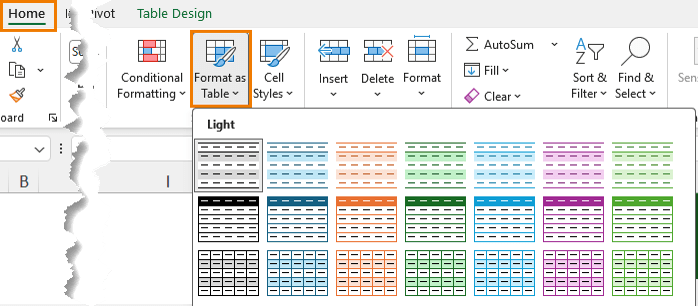
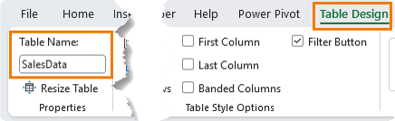
Choose a style and rename the table to something meaningful like: SalesData
Why this matters:
- Tables automatically expand when new data is added
- Formulas referencing tables update automatically
- Structured references make formulas easier to read
Keep your data and report on separate sheets. This keeps things clean and easier to manage.
Step 2: Create Dynamic Lists for Dropdowns
Most reports rely on dropdowns, but static lists require constant maintenance.
Instead, use formulas that update automatically.
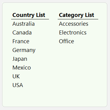
Country List
Use the UNIQUE function to extract distinct values:
=UNIQUE(SalesData[Country])
Wrap it in the SORT function for usability:
=SORT(UNIQUE(SalesData[Country]))
Now, when a new country is added to the data, it appears automatically.
Category List
Repeat the same process:
=SORT(UNIQUE(SalesData[Category]))
These two formulas replace manual steps like copying, removing duplicates, and sorting.
Step 3: Create Drop Down Lists That Update Automatically
Insert dropdowns using Data Validation: Data tab > Data Validation > List.
For the source, reference the first cell of your list and add the hash symbol:
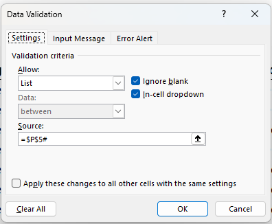
The hash symbol tells Excel to include the entire spilled range.
Repeat for the Category drop down.
This means:
- If the list grows, the dropdown grows
- If the list shrinks, the dropdown shrinks
No updates required.
Step 4: Build the Dynamic Report with FILTER
This is the core of the entire system.
The FILTER function extracts only the data that matches your criteria.
=FILTER(SalesData,
(SalesData[Country]=D4)*
(SalesData[Category]=D5),
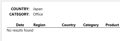
"No results found"
)
How This Works
Each condition (SalesData[Country]=D4) and (SalesData[Category]=D5) returns TRUE or FALSE for every row.
- TRUE = 1
- FALSE = 0
When you multiply conditions:
- TRUE × TRUE = 1 (row is included)
- FALSE × anything = 0 (row is excluded)
Multiplying conditions acts as an AND condition.
If you need OR logic, use a plus sign instead:
Condition1 + Condition2
This approach is powerful and reusable across many Excel functions.
Step 5: Create a Dependent Dropdown
Right now, your category list shows all categories, even those not relevant to the selected country.
You can improve this by filtering the category list to only include categories relevant to the country:
=SORT(
UNIQUE(
FILTER(SalesData[Category], SalesData[Country]=D4)
))
Now:
- Selecting Japan shows only relevant categories

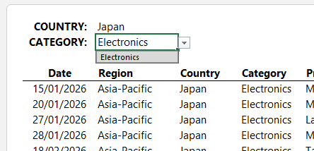
- Selecting another country updates the options instantly
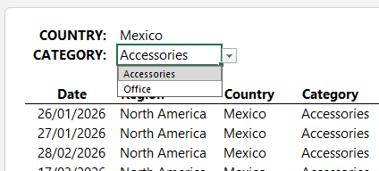
This is called a dependent dropdown.
Step 6: Add Summary Calculations
A good report shows key insights at the top.
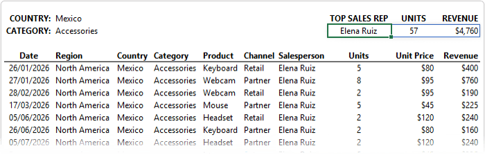
In this case, we want:
- Top salesperson
- Units sold
- Revenue
Use GROUPBY to aggregate data:
=IFERROR(
     TAKE(
       GROUPBY(
            CHOOSECOLS(C8#,7),
            CHOOSECOLS(C8#,8,10),
          SUM,
          0,
          0,
         -3),
       1),
   "")
What This Formula Does
- CHOOSECOLS selects relevant columns from the filtered data
- GROUPBY aggregates units and revenue by salesperson
- -3 sorts by the third column (revenue) in descending order
- TAKE returns the top result
- IFERROR handles empty results
This gives you the top performer instantly.
Why This Approach Works So Well
These four core functions work together:
- UNIQUE builds dynamic lists
- SORT keeps them user-friendly
- FILTER returns only relevant data
- GROUPBY summarises it
Once set up, the report becomes fully automated.
Add new data, and everything updates.
Common Mistakes to Avoid
1. The #SPILL! Error
This happens when something blocks a formula’s output range – take the screenshot below where the ‘x’ is inside the spill range.
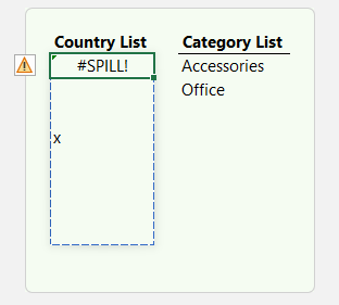
Fix it by clearing the cells in the spill area.
2. Using Tables for Spill Outputs
Dynamic array formulas do not work inside formatted Excel Tables.
Keep your results outside tables.
3. Using an Older Excel Version
These functions require modern Excel:
- FILTER: Excel 365 or 2021+
- GROUPBY, TAKE, CHOOSECOLS: Excel 365 or 2024+
If you do not see them in the IntelliSense when you type =FunctionName, your version does not support them.
Take It Further
This report is just one example of what Excel can automate.
Many repetitive tasks can be replaced with dynamic formulas like these.
If you want to build stronger Excel skills and learn techniques like this step by step, my Excel Expert course is designed to help you do exactly that.
Final Thoughts
Once you build a report like this, it changes how you use Excel.
Instead of rebuilding reports, you create systems that run themselves.
And once you start using dynamic arrays properly, going back to manual methods feels slow and unnecessary.
If you want to keep improving, the next step is learning more automation techniques you can apply every day.


genial, el informe dinámico sin aplicar las tablas, me gusta la forma que trasmite sus conocimientos, Felicitaciones Mynda
Muchas gracias, Viktor!
Excelente material claro, dinamico y de facil comprensión
Gracias!
thanks you are the 1 in excel for me i download the worksheet but id doesn’t work in the list to choose the country and category why?
Hi Bakir, great to hear you find our tutorials helpful.
I’m not sure what you mean by ‘but id doesn’t work in the list…’ as there is no ‘id’.
Mynda
Thanks, Mynda, for all your wonderful presentations. I have learned so many useful ways of working in Excel and love your creative examples. Keep up the excellent work.
Regards, Hughie.
Thanks for your kind words and support, Hughie!