Advanced Conditional Formatting in Excel Using Formulas

Most Excel users stick to built-in conditional formatting rules. A colour scale here, a “greater than” rule there.

But the moment you start using formulas, everything changes.

Formula-based conditional formatting allows you to highlight entire rows, flag missing data, catch errors, track deadlines, and more. All automatically and in real time.

In this guide, you’ll learn practical, real-world examples you can apply immediately to stop manually scanning spreadsheets for issues.

Excel Conditional Formatting Formulas Video

Get the Conditional Formatting Example File

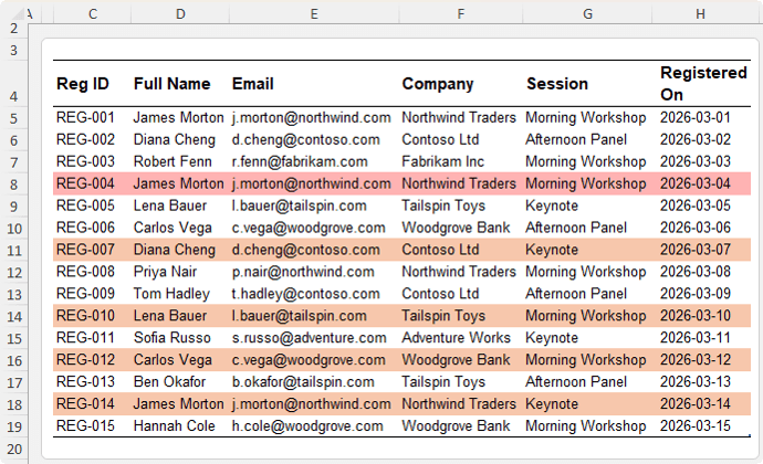
1. Format Entire Rows Based on One Cell

One of the most useful techniques is formatting an entire row based on a value in a single column.

Scenario

You have an orders table like this:

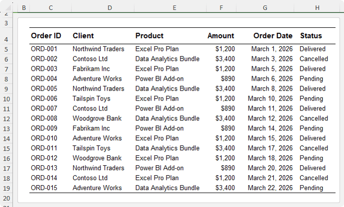
You want any row where the status is “Cancelled” to stand out.

Steps

1. Select the full data range
2. Go to Conditional Formatting → New Rule
3. Choose “Use a formula to determine which cells to format”
4. Enter this formula:

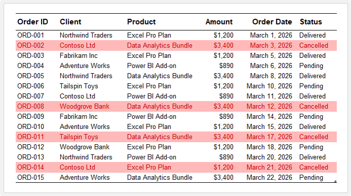
=$H2="Cancelled"

Key Concept

• The column is locked with $F so Excel always checks the Status column
• The row is relative so the rule evaluates each row individually

Now the entire row highlights when the status changes to Cancelled, and it updates instantly.

2. Compare Two Columns Automatically

Scenario

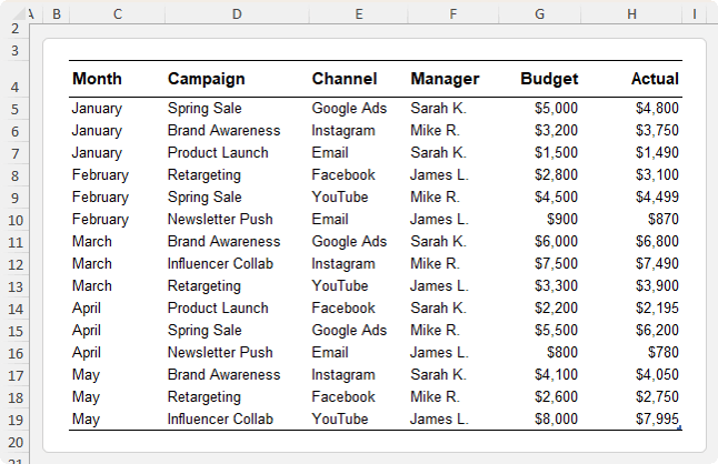
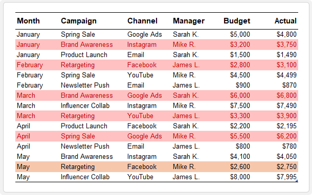
You want to flag rows where actual spend exceeds budget:

Formula

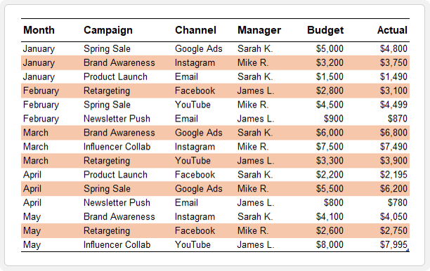
=$H5>$G5

This checks if Actual is greater than Budget.

Improve It with Thresholds

Add a second rule to highlight rows where spend is more than 10% over budget:

=$H5>$G5*1.1

Result

• Slightly over budget → one colour
• Significantly over budget → stronger colour

You can instantly identify problem areas without scanning numbers.

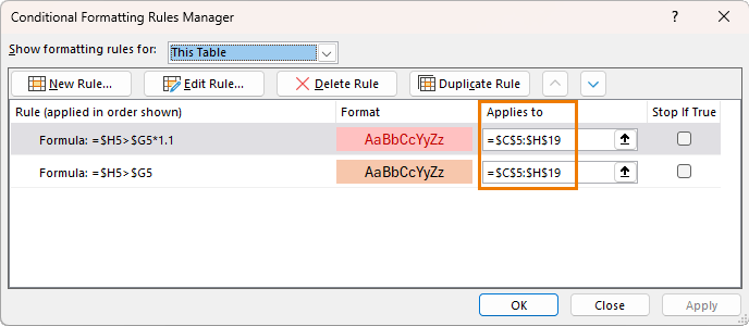
Important Tip

Use Manage Rules to control priority. Place the stricter rule above the general one so it takes precedence.

3. Flag Missing Data in Rows

This is one of the most practical rules you’ll use.

Scenario

You have a contact list with missing emails, phone numbers, or account managers:

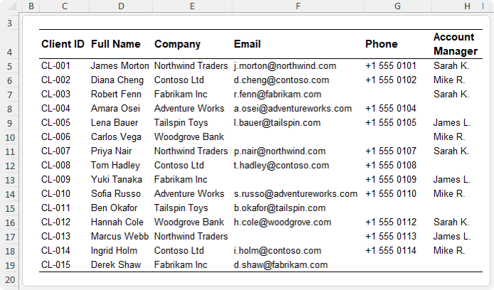
Formula

=SUM(--ISBLANK($C5:$H5))

How It Works

• ISBLANK checks each cell in the row
• It returns and array of TRUE or FALSE values, one for each cell in the row
• The double unary converts TRUE/FALSE to 1/0
• SUM adds them up to a single value required by the conditional format

Result

• If any cell is blank → result is greater than 0
• The row is highlighted

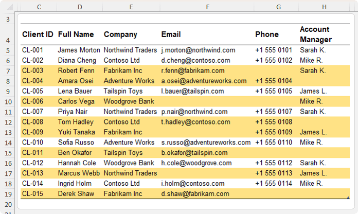
Fill in the missing data and the formatting disappears automatically.

4. Highlight Rows Containing Keywords

Scenario

You have a Comments column and want to find specific keywords like “urgent” or “burned out”.

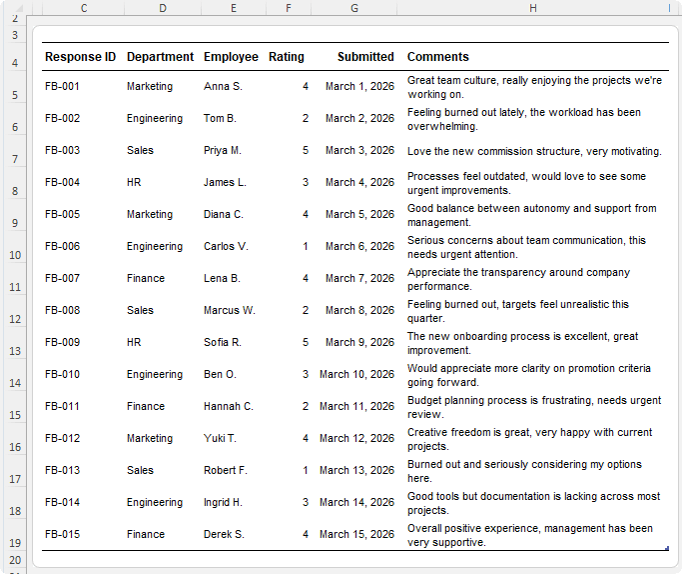
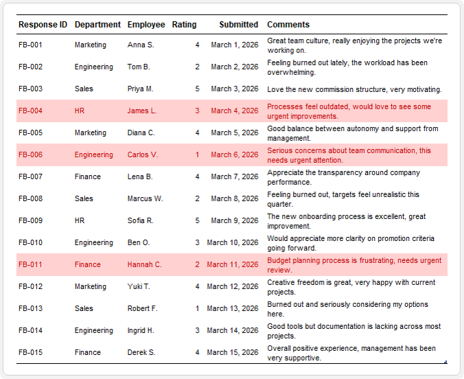
Formula for “urgent”

=SEARCH("urgent",$H5)

Why This Works

• SEARCH returns a number if the word is found (it is not case sensitive)
• It returns an error if not found
• Conditional formatting treats numbers as TRUE and errors as FALSE

Add Multiple Signals

Create another rule for “burned out”:

=SEARCH("burned out",$H5)

Result

• Urgent issues → one format
• Burnout mentions → another

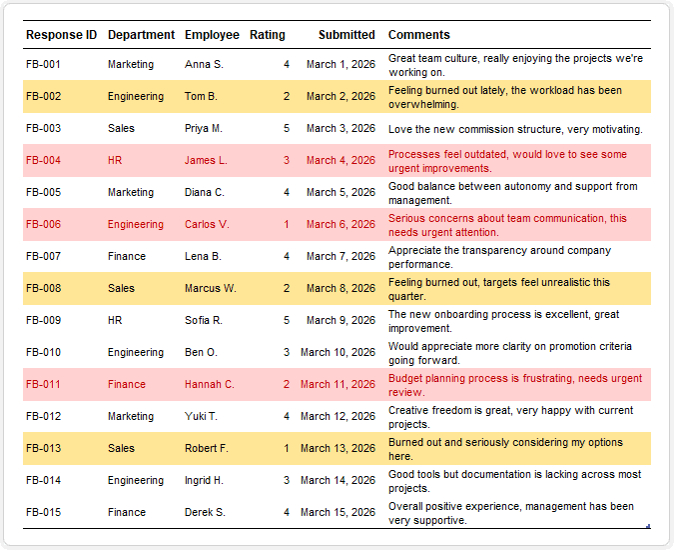
You can prioritise without reading every comment.

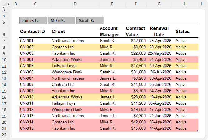
5. Create Date-Based Alerts That Update Automatically

Scenario

You manage contract renewals and need to know:

• What is overdue
• What is coming up soon

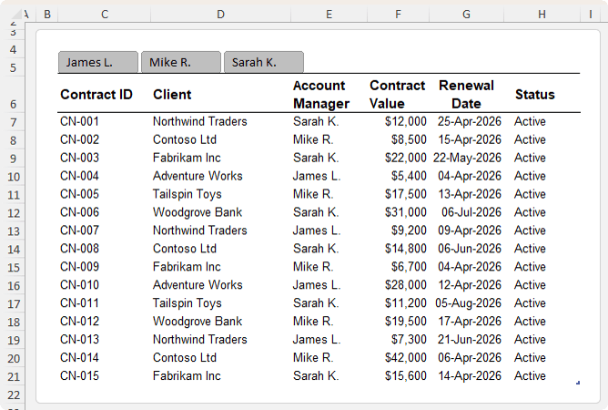
Overdue Contracts – format red

=$G7<=TODAY()

Contracts Due in Next 7 Days – format yellow

=$G7<=TODAY()+7

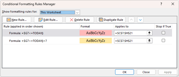
Key Benefit

The TODAY function recalculates automatically.

That means:

• A contract that was fine yesterday may be overdue today
• No manual updates required

Tip: Always set rule priority in the Conditional Formatting Manager so overdue items override upcoming ones:

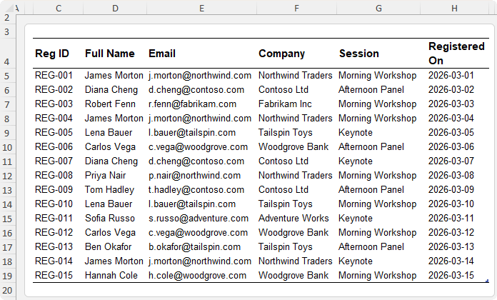
6. Detect Duplicates with Full Control

Excel has a built-in duplicate rule, but it flags both the original and duplicate.

Using formulas gives you more control. Let’s take the following data:

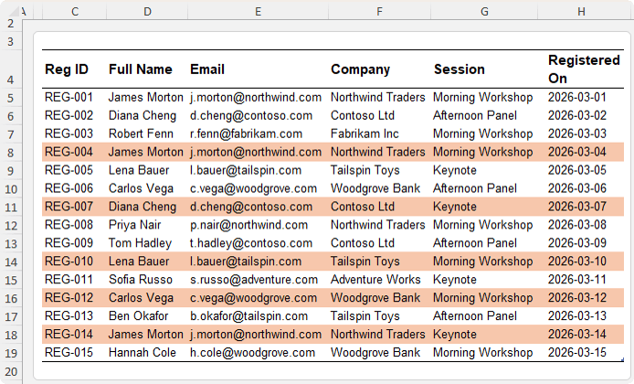
Highlight Only Duplicate Entries

=COUNTIF($E$5:$E5, $E5)>1

How It Works

• The reference $E$5:$E5 enables the range to expand as Excel moves down
• The first occurrence is counted once
• Counts of duplicates return a value greater than 1 and the format is applied

Result

• Original entry stays clean
• Only duplicates are flagged

Advanced: Match Multiple Columns

Use COUNTIFS to detect duplicate email and session combinations:

=COUNTIFS($E$5:$E5, $E5, $G$5:$G5, $G5)>1

Result

• Exact duplicates → stronger formatting
• Partial duplicates → lighter formatting

This creates a clear hierarchy of issues.

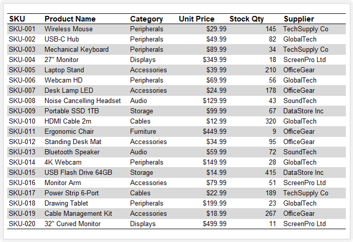
7. Create Banded Rows That Work with Filters

Excel Tables offer banded rows, but they limit some functionality like dynamic arrays, so we need an alternative approach.

You can recreate banding with conditional formatting.

Formula

=MOD(SUBTOTAL(3, $C$5:$C5),2)

How It Works

• The first argument of SUBTOTAL specifies the function: 3 is COUNTA. However, SUBTOTAL counts visible rows only
• This respects filters
• MOD alternates between 0 and 1

Result

• Every second visible row is formatted
• Banding adjusts automatically when filtering

This is far more flexible than standard table formatting.

Take Your Conditional Formatting Further

Everything in this guide builds on core Excel functions.

The more functions you know, the more powerful your conditional formatting becomes.

Functions like XLOOKUP, SUMIFS, and IF can be combined to create highly intelligent rules that adapt to complex data scenarios.

If you want to go deeper into formulas and unlock more advanced techniques, you can explore the full Advanced Excel Formulas course here.

If you start using these formula-based rules, you’ll spend far less time checking spreadsheets and far more time acting on insights.