The Excel INDEX function can lookup a range of cells and return any of the following:
- a single value
- an array of values
- a reference to a cell
- a reference to a range of cells.
It's this flexibility that makes it a truly powerful function, even if you only use it for the first option.
We’ll start with some straight forward examples and build from there, but first, the technicalities.
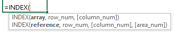
Excel INDEX Function Syntax
| Syntax 1: | =INDEX( array, row_num, [column_num]) |
Excel INDEX Function Arguments
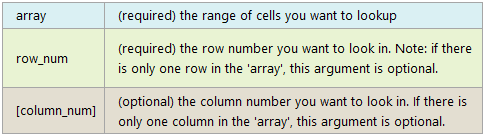
I’ll say this now, but don’t worry if it doesn’t resonate yet because I’ll show you an example later:
If the array has more than one row and more than one column, and only row_num or column_num is used, then INDEX will return an array of the entire row or column in the array argument.
Download the Workbook and Follow Along
Enter your email address below to download the sample workbook.
Excel INDEX Function Examples
We’ll start with a basic data table to use in the examples:
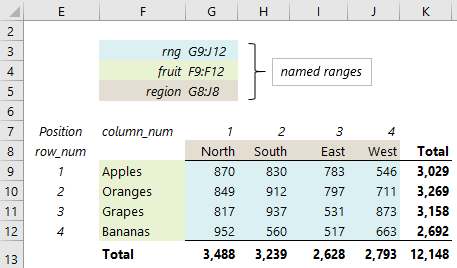
Note that the row labels, column headers and values areas all have named ranges which I’ll use in the formula examples. I’ve also added a total row and column, so you can cross reference the formula results to aid understanding.
INDEX Function Examples
Perhaps the most common use of the INDEX function is to lookup a value in a range (which is the array argument), and return a value from the corresponding row/column intersection. For example, let’s say I want to know the value for Grapes in the West region.
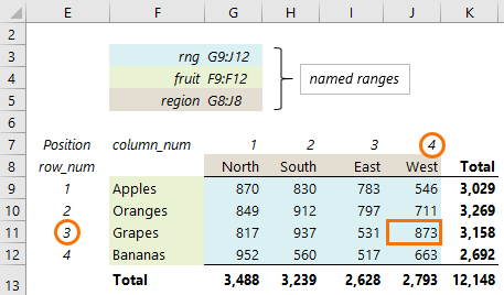
I could use this INDEX formula:
=INDEX(rng, 3, 4)
In English is reads, lookup the cells called ‘rng’ and return the value that at the intersection of row number 3, and column number 4.
=873
But if we already know that Grapes is in row 3 and West is in column 4, then we don’t really need INDEX, do we?
No, the real power comes when you use MATCH to find the row_num and column_num arguments like this:
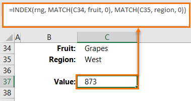
Formula in cell C37:
=INDEX(rng, MATCH(C34, fruit, 0), MATCH(C35, region, 0))
In English the above formula reads; lookup the rng and return the value at the intersection of the row that matches ‘Grapes’ in the ‘fruit’ range and the column that matches 'West' in the ‘region’ range.
Which evaluates to this:
=INDEX(rng, 3, 4)
=873
Note: If the row_num or column_num points to a cell outside of the array, INDEX will return the #REF! error.
Now that MATCH is doing the heavy lifting we can really put it to work with data validation lists that allow us to toggle through the different items like this:
Congratulations, you’ve just mastered INDEX & MATCH as an alternative to VLOOKUP.
More on the Excel MATCH function.
INDEX Single Row or Column
In certain circumstances the INDEX function’s row_num and column_num arguments are optional, namely:
If the array being indexed only contains a single column then there is no need for the column_num argument.
Obviously, you might say, but stick with me, there’s a twist.
For example, let's say we want to return the value in row number 2 of the Fruit range.
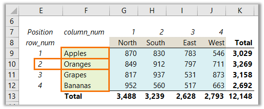
We can simply write the formula like this:
=INDEX( fruit, 2)
=Oranges
Likewise, if the array being indexed only contains a single row, there is no need for the row_num argument.
For example, let's say we want to return the value in column number 3 of the Region range (cells G8:J8).
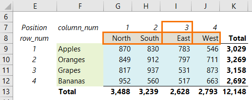
We can write the formula like this:
=INDEX(region, 3)
=East
Hold up! Did you notice the column_num argument, 3, is in the row_num argument’s position?
If you prefer to use a placeholder for the row_num argument you can add a comma to your INDEX formula like this:
=INDEX(region, , 3)
But, this extra comma is not strictly necessary as INDEX is looking up the array provided and returning the value in the third position, irrespective of whether the array is arranged in a row or column.
In other words, if your array is a single dimension, either a row or a column, then only one more argument is required for the position you want returned. And that argument can be placed in the row_num or column_num position of the formula.
But that’s not all folks, you can also write the formula like this:
=INDEX(region, 1, 3)
Of course, telling INDEX to return a value from row 1 of a single row array is an insult to its intelligence 😉.
Another option is to use zero for the row_num argument, like this:
=INDEX(region, 0, 3)
What? Row zero. Where is that? Well, when the row_num argument is zero, or empty, INDEX actually returns a reference to the whole column specified by the column_num argument. In this case the whole column is only 1 row high, or in other words, one cell; I8.
The inverse of this also applies; i.e. if your array is a column and you omit or use zero for the column_num argument.
Now, if you learn nothing more than the above points you’ll be way ahead of most Excel users. So, well done.
However, if you haven’t learnt anything new so far, or you’re eager to learn more, then keep reading because we’re going to start looking at the other 3 things the Excel INDEX function can do.
Return a Range with Excel INDEX Function
Expanding on the idea of omitting arguments or using zero for the row or column num arguments, let’s take a look at what happens when we reference the rng array.
I’ll repeat my earlier point; when a row or column num argument is omitted, or zero is used, INDEX actually returns a reference to the whole row or column.
However, typically INDEX is placed in a single cell and so when the range being returned is more than one cell, INDEX will return the #VALUE! error.
Let me illustrate these points with the following formula, which returns the second column of the cells named ‘rng’:
=INDEX(rng, ,2)
In other words, the above formula returns the range H9:H12.
There are 3 examples of this range being returned by INDEX in the image below:
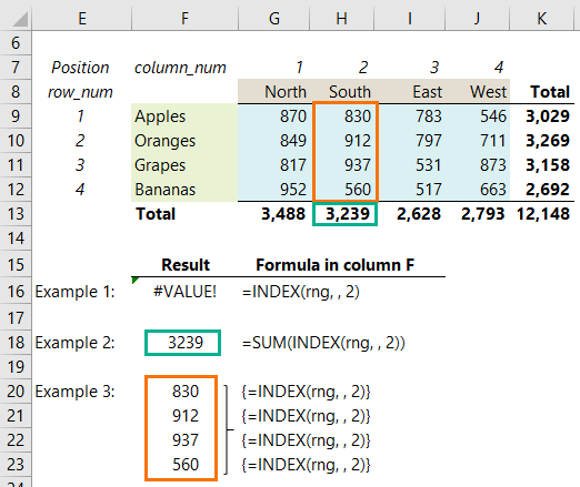
Example 1: Cell F16 - INDEX is entered in a single cell and returns the #VALUE! error. It’s returning the range H9:H12 and we haven’t told Excel what to do with that range, so #VALUE! is returned. We’d get the same error if we simply entered = H9:H12 into a cell.
Example 2: Cell F18 – INDEX is wrapped in the SUM function and returns the sum of the range H9:H12. It’s the same as entering =SUM(H9:H12) into a cell.
Example 3: Cells F20:F23 – INDEX has been array entered* into 4 cells which enables it to return the 4 values.
*To ‘array enter’ this formula, select the 4 cells (because the range H9:H12 is 4 cells high), then type the formula in and press CTRL+SHIFT+ENTER to complete the formula. This inserts the curly braces around the formula that you can see in the screenshot above, and places the 4 values in individual cells.
Notes:
- When you array enter the formula in example 1 (with CTRL+SHIFT+ENTER), it will return the first value in the range, i.e. 830.
- If you enter the formula in example 1 on rows 9, 10, 11 or 12, it will return the value on the corresponding row, as opposed to the #VALUE! error. This is due to implicit intersection.
Uses for INDEX Returning a Range
Extending what we know about INDEX being able to return a range, let’s look at some uses for this with a new data set shown below. Note the new named ranges; sales, dept and period.
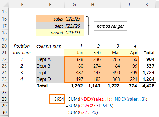
In cell F28 in the image above we can see the range being summed is returned by an INDEX formula on either side of the colon operator:
=SUM(INDEX(sales, ,1) : INDEX(sales, , 3))
It evaluates like so:
=SUM(G22:G25 : I22:I25)
In the next evaluation step Excel only keeps the extremities of the two ranges so we end up with:
=SUM(G22 : I25)
=3654
Now consider making the periods being summed dynamic. We can do this by replacing the column_num arguments with references to another cell that contains data validation lists that the user can choose from:
Most people use the OFFSET function to calculate dynamic named ranges, but INDEX is far more efficient and doesn’t suffer the volatility of OFFSET.
Excel INDEX Function – 4 Uses
Circling back to the 4 uses for INDEX, which were to return:
- a single value
- an array of values
- a reference to a cell
- a reference to a range of cells.
Have you made the connection that 1 and 3 are the same thing, and 2 and 4 are the same thing? And whether you get a value/values or a reference simply depends on how you use INDEX.
For example, the following formula:
=INDEX(sales, 1, 1)
Returns the reference to cell G22:
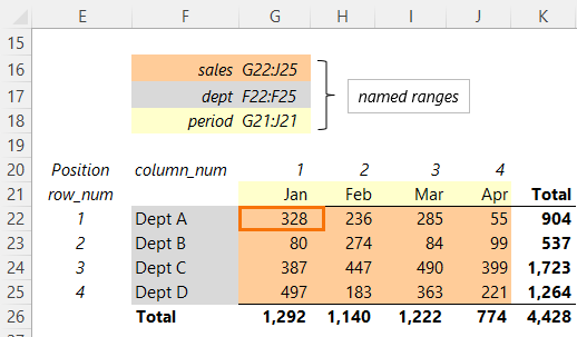
If you enter the above formula in an empty cell it will display the value from cell G22; which is 328.
But if you enter this INDEX formula nested in another formula, it will return the cell reference.
=COUNT(INDEX(sales, 1,1))
=COUNT(G22)
=1
More on dynamic named ranges here.
Referencing Non-contiguous Ranges
You may have noticed that INDEX has two syntax options:
The first one returns an array (single or multiple values), and the other returns a reference to a cell, or range of cells.
You don’t actually choose which syntax to use, Excel will decide that based on the inputs and the context of the formula. For example; whether the formula is entered in a single cell, nested inside another function, array entered etc.
So far, we’ve covered scenarios where the array or reference is a single contiguous range. So, let’s look at the second one which allows you to work with non-contiguous ranges.
Excel INDEX Function Syntax – Non-contiguous Ranges
| Syntax 2: | =INDEX( reference, row_num, [column_num], [area_num]) |
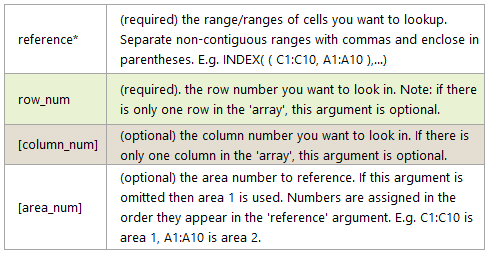
*References must be on the same sheet, otherwise the #VALUE! error is returned. References can be different shapes/sizes, but if the row_num or column_num argument refers to a row or column outside of the reference area, INDEX will return the #REF! error.
INDEX Non-contiguous Range Examples
In the screenshot below we have two sets of stores; Stores A to D and Stores E to H. Just imagine there are two managers responsible for these two store groups and that’s the reason for their separation.
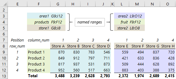
Let’s say we want to find the value for Product 4 in Store G. We’d use this INDEX formula:
=INDEX((area1, area2), 4, 3, 2)
=388
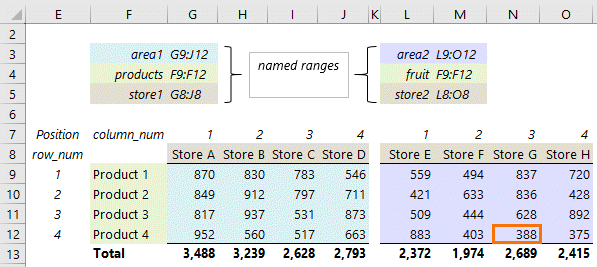
Notice the two references are separated by a comma and wrapped in parentheses:
=INDEX( (area1, area2), 4, 3, 2)
Remember, the references must be on the same sheet, otherwise INDEX will return the #VALUE! error.
Reference a Whole Column or Row
We can also return a reference to a whole row or column. For example, if I want to sum the values for store G, I can put a zero in the row_num argument like this:
=SUM(INDEX((area1, area2), 0, 3, 2))
=2,689
And I can sum Product 4 for Area 1 like this:
=SUM(INDEX((area1, area2), 4, 0, 1))
=2,692
Notice that it doesn’t sum all of Product 4, only that of area 1.
Excel INDEX Function Limitations
It's such a versatile function and there aren’t many limitations. Perhaps the main limitation is the requirement that the reference ranges must be on the same sheet. The workaround to this is to use a different function to return the reference.
The Excel CHOOSE function is a great alternative:
=SUM( INDEX( CHOOSE( 1, area1, area2), 4, 0) )
=SUM( INDEX( area1, 4, 0) )
=2,692
Notice that instead of this:
=SUM(INDEX((area1, area2), 4, 0, 1))
We have this:
=SUM( INDEX( CHOOSE( 1, area1, area2), 4, 0) )
Related Functions
| MATCH Function | The MATCH function looks up a value in a range and returns the relative position of that value. |
| OFFSET Function | The OFFSET Function returns a range of cells offset from a starting cell. |
| Dynamic Named Ranges | Dynamic named ranges automatically update based on criteria you specify. |
| CHOOSE Function | The CHOOSE Function returns a value or range from a list based on the position specified. |
| VLOOKUP Function | The VLOOKUP function looks up a value in a column and returns a corresponding value from a column to the right. |
| HLOOKUP Function | The HLOOKUP function looks up a value in a row and returns a corresponding value from a row below. |
Excel INDEX Function Formula Examples
Dynamic Dependent Data Validation
Excel Find Column Containing a Value
Return the First and Last Values in a Range
Locating Values in Large Excel Tables
Excel Remove Blank Cells from a Range
Lookup and Return Multiple Matches