Excel VLOOKUP with Dynamic Column Reference

If you ever work with large tables of data and you want to insert a VLOOKUP formula that dynamically updates to the next column as you copy it across, then the VLOOKUP with the COLUMNS function is what you need.

That is; the col_index_num part of the VLOOKUP function dynamically updates as you copy it across your worksheet.

=VLOOKUP(lookup_value,table_array,col_index_num,[range_lookup])

For this example I downloaded the current top 10 selling books from Amazon – see below.

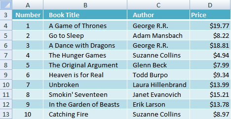
Book number 2 sounds like it might have some tips for getting my two boys to bed…must put it on my shopping list…… Sorry, I digress.

Ok, let’s imagine this list is hundreds or even thousands of rows long and we want to find a quick way to get prices and author information on demand (other than CTRL+F for Find of course).

In the table below we have the Book Title, Author and Price.

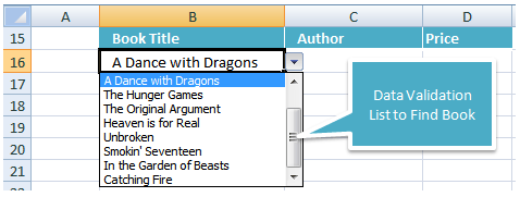
The book title is found using a Data Validation List or Drop Down List, and in column C and D we need a VLOOKUP formula that finds the Author and Price respectively.

We could do this using an ordinary VLOOKUP formula like this:

In cell C16 =VLOOKUP($B16,$B$4:$D$13,2,FALSE)

And in cell D16 =VLOOKUP($B16,$B$4:$D$13,3,FALSE)

But we need to manually edit the column reference for each column we copy the VLOOKUP across to.

Go here for a refresher on the VLOOKUP function.

And if we’ve got a lot of columns that we want to look up, then instead of hard coding the column reference number it’s much quicker to use the COLUMNS function like this:

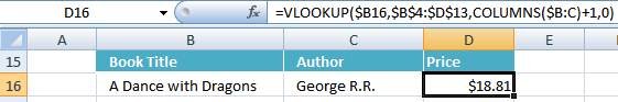
In cell C16 =VLOOKUP($B16,$B$4:$D$13,COLUMNS($B4:B4)+1,0)

And in cell D16 =VLOOKUP($B16,$B$4:$D$13,COLUMNS($B4:C4)+1,0)

Note: Make sure you use the COLUMNS (plural) not COLUMN as they work quite differently.

What’s going on with the COLUMNS function?

The COLUMNS function returns the number of columns in an array.

The syntax is =COLUMNS(array), where ‘array’ is the column range. For example:

=COLUMNS(B4:B4) gives us 1 i.e. the array is 1 column wide.

So all we’re really doing is calculating the column number we want using the COLUMNS function.

Note: B4:B4 could just as easily been plain B:B like this =COLUMNS(B:B), as it doesn’t really matter what the row reference is.

VLOOKUP using COLUMNS Function Explained

In our VLOOKUP formula above (in cell C16), our COLUMNS formula is COLUMNS($B4:B4)+1, because:

1.       the column we want returned is the second column in our VLOOKUP table,

2.       and since =COLUMNS($B4:B4)  evaluates to 1 we need to add 1 to get 2 for the second column.

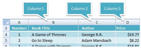
In our VLOOKUP formula in cell D16 our COLUMNS function is COLUMNS($B4:C4)+1 and it evaluates to 2+1=3

We’ve used an absolute cell reference on $B4:C4 (=2) so that when we copied the VLOOKUP formula across from C16 to D16 the COLUMNS part of the formula will automatically increase by 1 (from B4:B4 to B4:C4) to give us the correct column number.

Alternative to using COLUMNS is the MATCH function

As an alternative in my INDEX MATCH tutorial I show you how you can use the MATCH function to create a dynamic column reference.  Just another way to skin a cat.

The limitation of the MATCH function used this way is that the VLOOKUP formula and the table_array must contain column headers that are the same.

See example towards bottom of INDEX MATCH tutorial.

HLOOKUP with ROWS

Similar to using VLOOKUP and COLUMNS, we can use the ROWS function with HLOOKUP to achieve the same effect, but for the row number.

Syntax for ROWS function:

=ROWS(array) where ‘array’ is the row range. For example:

=ROWS(B4:B4) gives us 1 i.e. the array is 1 row high.

I think you get the idea, but if you’re not familiar with HLOOKUP you can read my HLOOKUP tutorial and insert the ROWS function in place of the row number in the HLOOKUP formula just as we did for the column numberin the VLOOKUP above.

Download the workbook and reverse engineer the formulas or practice what you learn.

Want more? Sign up for our newsletter below and receive weekly tips & tricks to your inbox, plus you’ll get our 100 Excel Tips & Tricks e-book.

Tagged as: vlookup