Excel HLOOKUP Formulas Explained

HLOOKUP is just like the VLOOKUP formula only the table you are looking up is laid out in a horizontal list, rather than vertically.  Hence the ‘H’ for horizontal, and ‘V’ for vertical.

Just like the VLOOKUP, the HLOOKUP can be used to find an exact match or used in a sorted list.

Download the workbook and practice what you learn, or reverse engineer the formulas for deeper understanding.

We’ll look at a HLOOKUP Exact Match scenario first.

HLOOKUP Exact Match

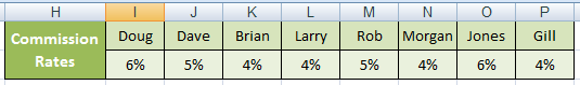
In the table below we want to calculate a commission in column F for each builder.  We have each builder’s specific commission rate in a horizontal table in columns H to P, and we’ll use the HLOOKUP formula to calculate our commission.

Microsoft Excel describes the HLOOKUP formula as:

HLOOKUP(lookup_value, table_array, row_index_num, range_lookup)

And to translate it into English it would read:

HLOOKUP(find this value, in that table, return the value in row x of the table, but only return a result if you can match the value exactly)

Let’s make it even clearer by applying it to our example:

HLOOKUP(find Doug in cell B2, in the Commission Rates table I1:P2, return the value in row 2 of the table,  and only return a value if you find Doug in the Commission Rates table otherwise give me an error)

Firstly let me make a few things clear:

1)     ‘Return the value in row 2 of the table’ is referring to the row number in the table I1:P2, not the row number of the spreadsheet, even though in this example they are the same.

2)      ‘Only return a result if you can match the value exactly’ is instructing Excel that we only want information returned if it matches our criteria exactly.  i.e. Find Doug in our Commission Rates Table, and if you can’t find Doug, give me an error.  The error displayed will be #N/A.

On the other hand, if we told Excel it was ok to not find an exact match, it would return the next best result.  i.e. If Doug wasn’t in our table Excel would return the next best result.  In this scenario we wouldn’t want it to do that, but this option is handy in other situations which we’ll cover later in this tutorial.

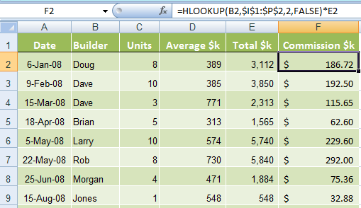
OK, now that’s clarified, in Excel our HLOOKUP formula in column F for the above example would be:

=HLOOKUP(B2,$I$1:$P$2,2,FALSE)

Note: you’ll notice the table range I1:P2 has dollar $ signs around it.  For more on this read my previous tutorial on absolute references.

This would give us the commission rate for Doug of 6%, but what we really want in column F is the commission $ amount.  This is easily achieved with an extension to the above formula as follows.

=HLOOKUP(B2,$I$1:$P$2,2,FALSE)*E2     (with E2 being the Total $k)

Let’s make it even easier by giving the Commission Rates table a named range.  Let’s call it ‘ComRates’.  We could then more easily build the HLOOKUP formula, and also interpret it quickly when revisiting the worksheet at a later date.  With a named range of ‘ComRates’ our HLOOKUP formula would read:

=HLOOKUP(B2,ComRates,2,FALSE)*E2

HLOOKUP Sorted List

The Sorted List version of the formula looks almost the same up to the last argument ‘FALSE’.  In a Sorted List HLOOKUP formula you can either leave this last argument blank, or enter ‘TRUE’.

Although the formula looks the same when you use ‘TRUE’, HLOOKUP finds the nearest match for the value you’re looking up.  Let’s look at an example.

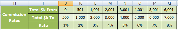
Using the previous example, again we want to calculate the Commission $ amount.  However, this time the commission is based on the Total $k amount and where it falls into our Commission Rates table.

As a result our Commission Rate is based on where the Total $k falls into the scale on our table.

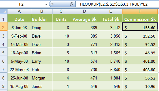
Taking the table below our HLOOKUP sorted list formula for column F in English will read:

=HLOOKUP(Find the Total $k in cell E2, in the commission rates table, return the value in row 3 of the table, if you can’t find the exact amount go to the next lowest amount)

In Excel our HLOOKUP formula will be entered as follows (including the *E2 to get the actual $k commission amount as we did above):

=HLOOKUP(E2,$J$1:$Q$3,3,TRUE)*E2

Note: Excel doesn’t actually take into consideration row 2 in our Commission Rates table.  I have simply put it there to help understand the commission ranges.  Excel is in fact looking for the exact Total $k amount in our Commission Rates table, but when it can’t find it, it finds the next best lower amount and returns the value in row 3.

HLOOKUP Rules & Common Mistakes!

1)      HLOOKUP formulas read from top to bottom.  You must have the information you are looking up, in a row above the information you want returned.

2)      You can have as many rows as you like in your table, just so long as you follow the ‘top to bottom’ rule above.

3)      The ‘Table’ you are looking up can be in the same spreadsheet, or same workbook on a different sheet, or a different workbook altogether.

4)      If you find Excel is telling you it can’t find the value you’re looking up in your table by returning a #N/A result, but you can ‘plain as day’ see they’re both there.  It’s likely you’ve got one formatted as text and another formatted as general.  To check this go to each cell and look in the formula bar to see if one is prefixed by an apostrophe ‘.

5)      For the Exact Match version of the formula the table doesn’t have to be sorted in any particular order, but you must not have duplicates, unless the information on each duplicate is exactly the same.  For example, if Doug appeared twice in our Commission Rates table with different percentage rates for each instance, Microsoft Excel would return the rate on the first instance of Doug.

6)      For the Sorted List version of the formula; if we had duplicates in our Commission Rates table Excel will find the last instance of the value and return the result in row 3.  For example, if instead of the amount $2,001 in cell M1, you had $1,001 again.  Excel would return the value of 4% as it’s finding the last best match for our amount.  The tip here is to remove any duplicates or you’ll end up with erroneous results.

7)      The HLOOKUP Sorted List version of the formula requires the list to be sorted in ascending order from left to right.  If it’s not sorted you end up with nonsense.

Do you prefer VLOOKUP or HLOOKUP? Let us have your comments.

Share the knowledge with your friends and colleagues on Twitter, and Facebook etc. using the shortcuts below.

Tagged as: hlookup, lookup, vlookup