Must-know Excel Features

Even if you use Microsoft Excel daily, you may not be leveraging some of its best time-saving tools. In this blog post, we'll explore seven overlooked must-know features that can significantly reduce the time you spend on repetitive tasks. Try these out yourself using the example file provided!

Must-know Excel Features Video

Get the Practice File

1. Formula Auditing Tools

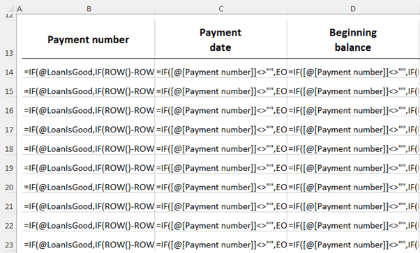
Imagine opening a complex spreadsheet filled with intricate formulas. It's overwhelming, right? Instead of spending time clicking through cells to understand their relationships, use Excel's Formula Auditing Tools:

• CTRL+`: This shortcut toggles between showing and hiding formulas in the entire worksheet. It gives you a quick overview of which cells contain formulas.

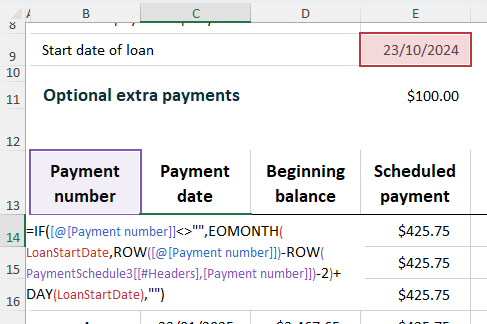
• F2: Pressing F2 while in a cell highlights and color codes the referenced cells, making it easier to trace inputs.

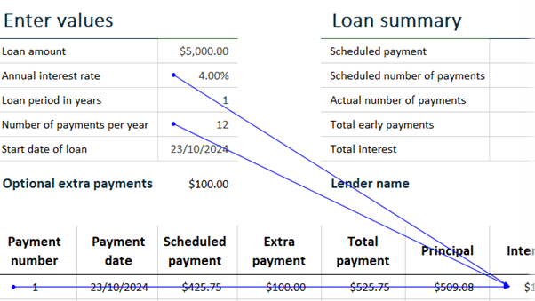
• Trace Precedents/Dependents: Go to the Formulas tab and use these options to visually map out cells linked to the formula you are inspecting.

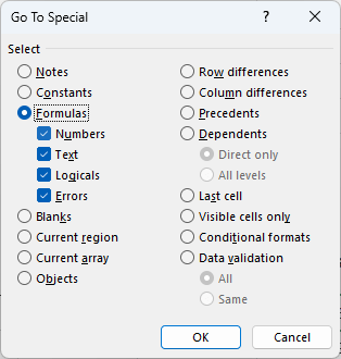
• Go To Special (CTRL+G): Identify all cells with formulas by choosing Special > Formulas. You can even filter by numbers, text, logical values (TRUE/FALSE), or errors.

These tricks help you quickly familiarize yourself with complex files, so you can spend less time investigating and more time solving problems.

2. Advanced Data Entry Settings

Data entry can be tedious, but Excel offers settings to make it efficient:

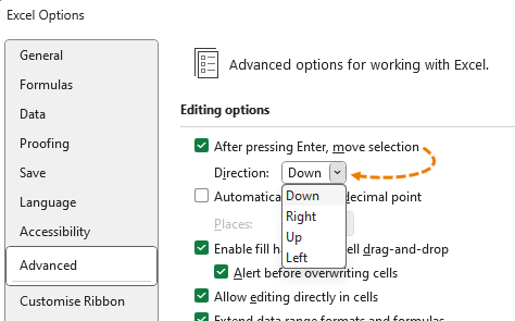
• Customizing Enter Key Behavior: By default, pressing Enter moves the cursor down. If you prefer moving right, go to File > Options > Advanced and change the direction under "After pressing Enter, move selection". This small adjustment saves time, especially when entering data in rows.

• Automatically Insert Decimal Points: If you're entering a lot of numbers with consistent decimal places, use File > Options > Advanced and select Automatically insert a decimal point.

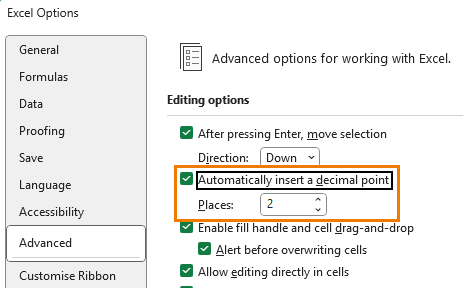
Specify the number of decimal places, and Excel will insert them as you type, speeding up data entry.

These tweaks might seem minor, but they can significantly enhance your workflow, especially for large data sets.

3. Find and Replace Formatting

Formatting changes across multiple cells can be time-consuming. Instead of manually updating each cell, use Find & Replace for a quick solution:

1. Press CTRL+H to open Find & Replace.
2. Click Format in both the Find and Replace sections to choose specific formatting attributes.

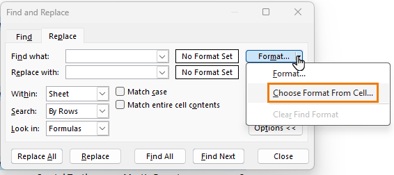
3. Apply the formatting changes (e.g., changing font, fill color, or borders etc.) across multiple cells instantly.

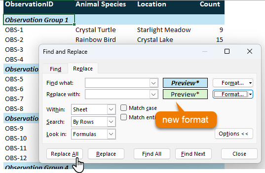
This method is particularly useful for applying consistent styles throughout large reports or datasets, ensuring everything looks polished in seconds.

4. Custom Ribbon Tab

Navigating Excel's ribbon to find frequently used commands can be a hassle. Save time by creating a Custom Ribbon Tab:

1. Right-click the Ribbon and select Customize Ribbon.
2. Add a New Tab and a New Group under it.

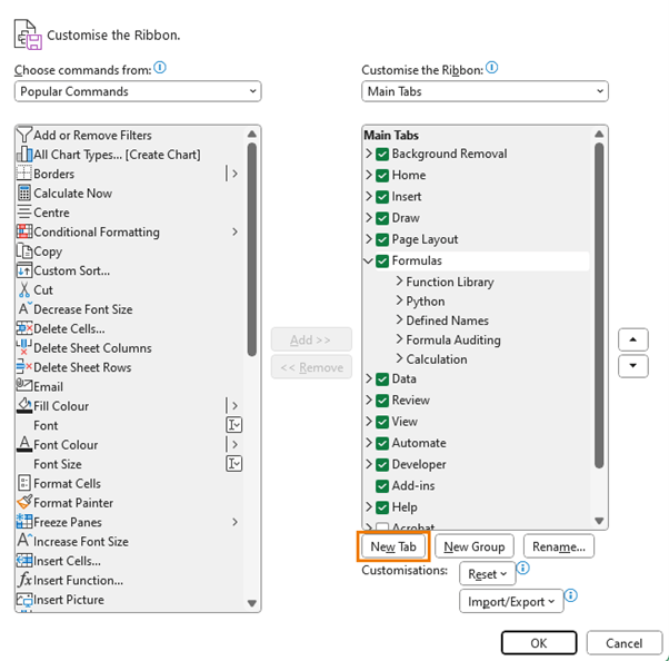
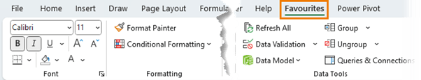
3. Rename the tab (e.g., "Favorites") and add frequently used commands or groups from the left pane, such as formatting tools or PivotTables.

This allows you to access your most-used tools in one place, boosting your productivity by minimizing the time spent hunting through different tabs.

5. Data From Picture

Ever wished you could pull data from a printed table or screenshot directly into Excel? You can with Data From Picture:

1. Copy an image of the table to your clipboard.
2. Go to the Data tab and select From Picture.

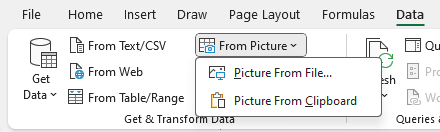
3. Choose From Clipboard or browse to a file, and Excel will process the image, converting the data into a worksheet format.

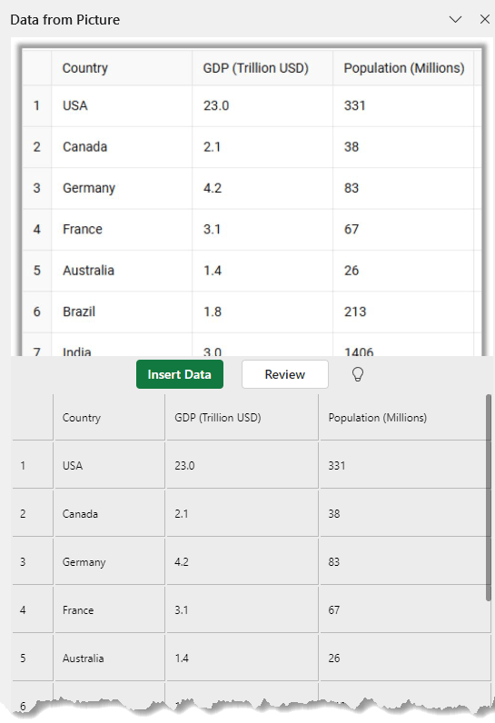
Review any highlighted cells for errors before inserting the data. This tool is perfect for quickly digitizing printed data without the need for manual entry.

6. Focus Cell

If you work with large spreadsheets, the Focus Cell feature (available in Microsoft 365 for Windows beta) highlights the row and column of the selected cell, making it easier to trace data across large ranges:

• Activation: Go to the View tab and select Focus Cell or use the shortcut ALT, W, E, F.

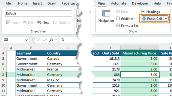
• Customize Colors: You can adjust the colors using the cell or font color palettes to make them more visually distinct.

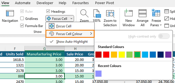
Tip: any custom colours you create in other colour palettes in Excel will be included in the 'Recent Colours' list here.

Although Focus Cell currently doesn't work with Freeze Panes or Split Panes, it's still an invaluable tool for quickly locating and verifying data.

7. Sparklines

Sparklines are mini charts that fit within a cell, making it easy to visualize trends without cluttering your worksheet with large graphs:

1. Select the cells where you want sparklines.
2. Go to the Insert tab and choose Sparklines (Line, Column, or Win/Loss).

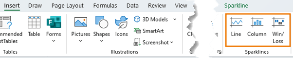
3. Select the data range, and Excel will insert these mini charts.

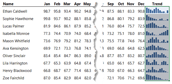
These compact visuals are perfect for time-based data, providing quick insights into trends without the complexity of full-sized charts.

Unfortunately, Sparklines can only display the trend for one series, but sometimes you might want to compare a value to a target, like actual costs versus budget, etc. and this is where my mini chart technique shines. So, check out this video next on inserting mini charts into cells so you aren't restricted by the limitations of sparklines.

Next Steps

These must-know Excel features are designed to make your work faster and more efficient. From data entry tricks to advanced formula tools, incorporating them into your workflow can save you hours each week. Try them out and see how much time you can reclaim!

Looking for more Excel tips? Check out our Excel Expert course that includes real-world examples and practice files, plus support and mentoring when you need it most.