Common Excel Mistakes

Many Excel users are confident in their skills, but Excel's vast functionality means it's easy to overlook some useful features. These overlooked features can lead to inefficiencies, making tasks more time-consuming than they need to be.

The good news? With a few quick adjustments, you can streamline your workflow and make Excel work smarter for you. Let's explore some simple changes that can boost your efficiency and accuracy.

7 Common Excel Mistakes Video

 

Get the Excel Workbook and Cheat Sheet

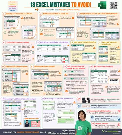
The free cheat sheet contains the 7 mistakes listed here and a bonus 18 more you can make sure you avoid.

Mistake 1. Manually Editing Cell References

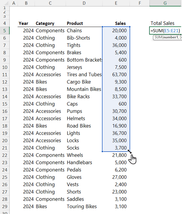
If you're constantly updating formula ranges:

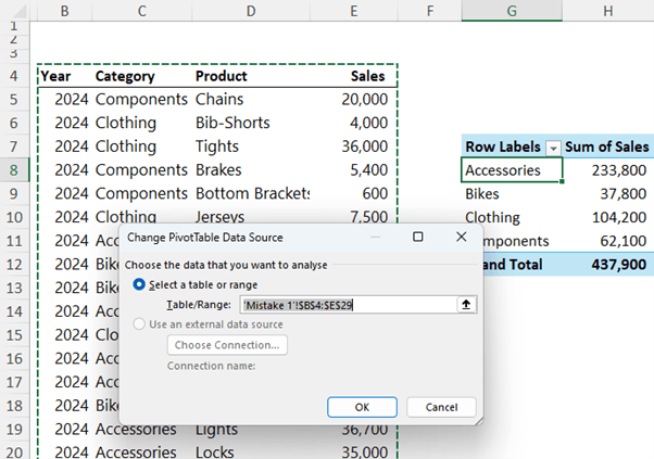
Or manually adjusting PivotTable sources:

Then you're missing out on a simple yet powerful Excel feature—Excel Tables.

The Fix:

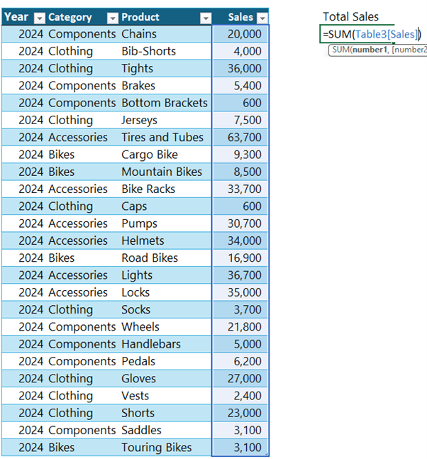
Transform your data into a Table using the shortcut CTRL+T. When you do this, Excel automatically updates formula ranges whenever you add new data.

By using structured references (like table names and column names) in your formulas, you ensure everything stays up to date, reducing the chance of missing data in reports.

And PivotTables update with the click of the Refresh All button:

Mistake 2. Complicated Running Total Formulas

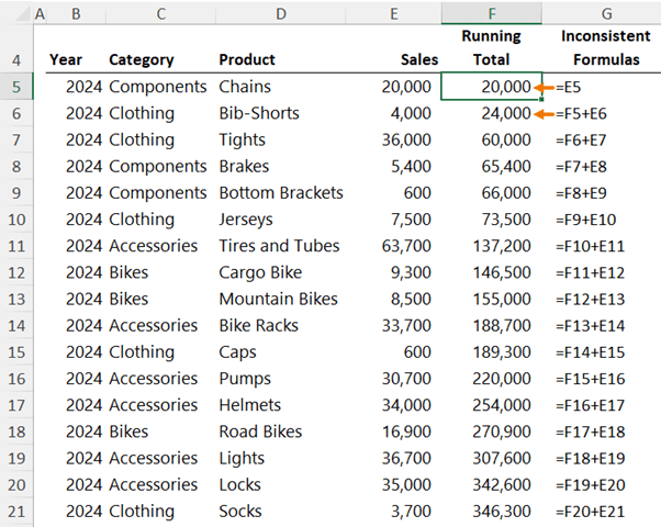
Many users create running totals where the formula in the first cell is different from the rest. For instance, the first cell may display a single value, while subsequent cells sum the previous and current values.

While this works, it's not efficient and can be risky since consistency in formulas is key to avoiding errors.

The Fix:

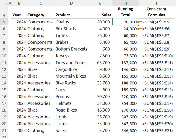
Use the SUM function with an absolute reference for the starting cell and a relative reference for the ending cell. For example:

This approach allows you to drag the formula down the column without needing any adjustments, ensuring consistency.

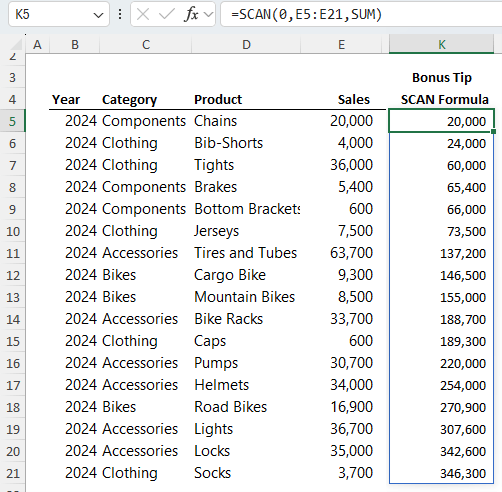
Bonus tip: Microsoft 365 users can also use the new SCAN function:

=SCAN(0,E5:E21,SUM)

Mistake 3. Manually Creating Numbered Lists

Typing numbers manually or maintaining a list yourself is both time-consuming and prone to error. Thankfully, Excel has a function designed for this.

The Fix:

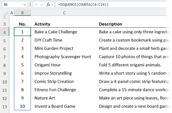
Use the SEQUENCE function. For example:

=SEQUENCE(COUNTA(C4:C17))

This formula generates a list that automatically updates as you add or remove items, keeping everything neat and dynamic.

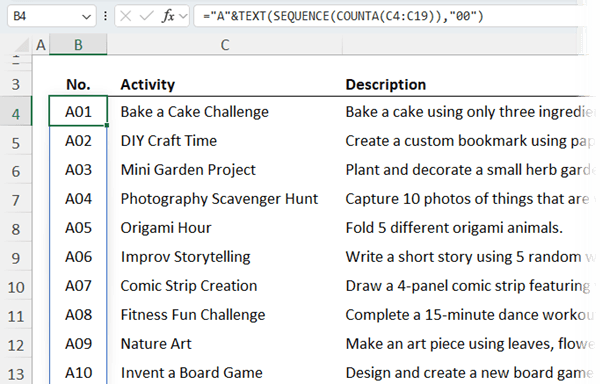
If you prefer an alpha-numeric sequence (like A01, A02), combine SEQUENCE with TEXT:

="A"&TEXT(SEQUENCE(COUNTA(C4:C17)), "00")

This formula creates a customizable format that adapts as your list grows.

Mistake 4. Listing Dates Manually

Manually entering dates is a tedious task, especially for longer periods. It's also unnecessary when Excel can automate the process for you.

The Fix:

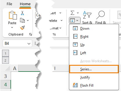
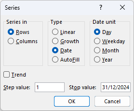
Use Excel's Fill Series tool to generate a list of dates.

Enter the start date, navigate to Home > Fill > Series, and set your preferred interval (days, weekdays, months, etc.).

Alternatively, you can use the SEQUENCE function with the DATE function:

=DATE(2024, 10, SEQUENCE(31))

This formula will return all dates for October 2024. Adjust the parameters to fit your needs, and Excel takes care of the rest.

Want month end or month start dates? Team SEQUENCE with the EOMONTH function like so for month end dates:

=EOMONTH(DATE(2024,1,0),SEQUENCE(12))

And like so for month start dates:

=EOMONTH(DATE(2023,12,0),SEQUENCE(12))+1

Mistake 5. Manual PivotTable Grouping

Excel's PivotTables group data into days, months, quarters, and years by default. However, many users add extra columns to their data to group it by weeks or other intervals manually.

The Fix:

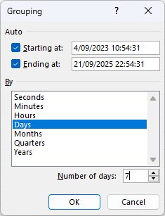
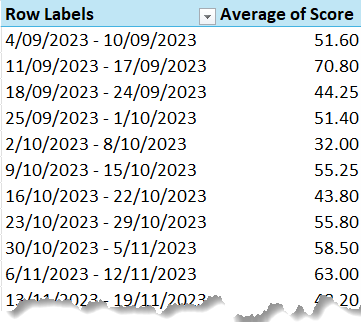
You can group dates by weeks directly in the PivotTable. Simply right-click the PivotTable date field and ungroup any existing grouping, and then right-click and Group > Days, setting the interval (e.g., 7 for weekly, 14 for bi-weekly).

And just like that you have your data grouped into weeks. The Starting at and Ending at dates are based on your dataset, but you can edit them in the dialog box above as required.

This eliminates the need for additional columns, making your dataset cleaner and your PivotTable setup more efficient.

Mistake 6. Using Merged Cells

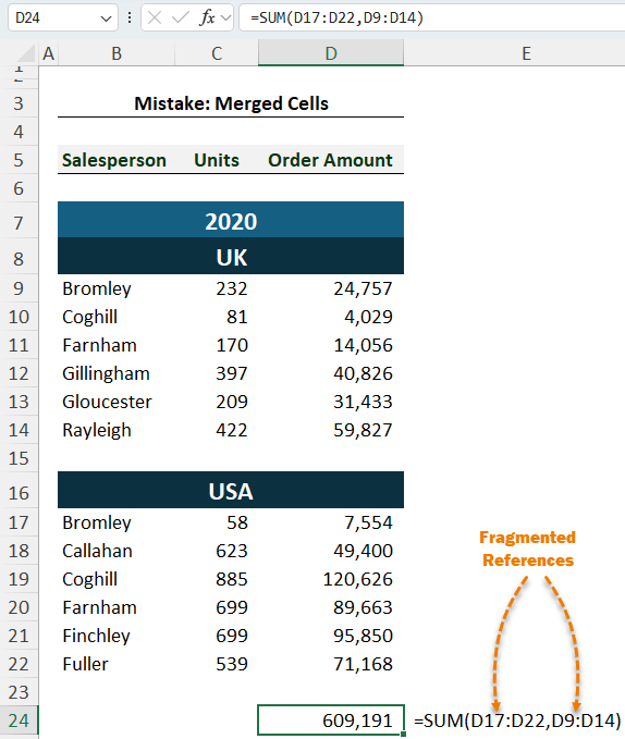
If you've ever had Excel refuse to sort or filter data, merged cells are likely the culprit.

While merging cells may seem like a good way to format your sheets, they create problems for data manipulation.

The Fix:

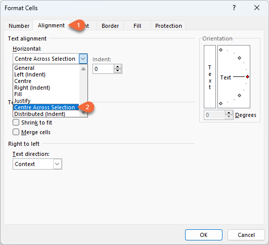
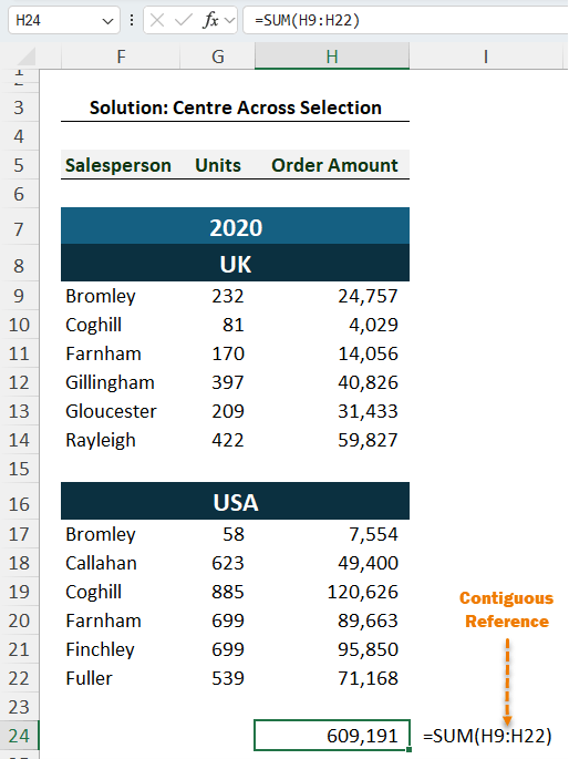
Instead of merging cells, use 'Center Across Selection' (CTRL+1 for the format menu).

This method centers your content without merging cells, allowing you to freely sort, filter, or sum columns without error.

Mistake 7. Wrapping Text the Wrong Way

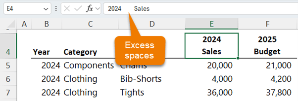
When you want to wrap text in cells (like for column headers), the common mistake is to add spaces manually to force the wrap.

Not only is this inefficient, but it can also create alignment issues.

The Fix:

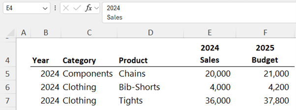
Use ALT+Enter to insert a line break directly in the cell. Make sure 'Wrap Text' is enabled, and you'll get neatly wrapped text without extra spaces.

This approach keeps everything consistent and easy to manage, especially when viewing or printing your sheets.

Bonus Tip

If you're ready to take your Excel skills even further, consider enrolling in one of our Excel courses.

You'll find hands-on lessons covering everything from the basics to advanced techniques that can save you hours of work. Plus, personal support and mentoring are available to help you master Excel and become an expert.

Excel is a powerful tool, but even experts can fall into these common traps. By avoiding these mistakes, you'll work more efficiently and accurately. Want more Excel tips and tricks? Check out our other blog posts and tutorials to keep learning!