How to Clean Data in Excel

Sending out a report that contains errors is embarrassing. I know, I've done it! You present a report to management, and they come back with questions around errors you should have found.

In this post I'll share 11 essential steps for pristine data to ensure it doesn't contain duplicates, extra spaces, misspelt words, and other more sneaky data anomalies that undermine your work.

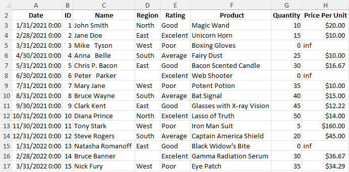
We've got a dataset that's a bit on the wild side, with all sorts of common issues. But don't worry, we'll tackle this together, starting with the basics and moving up to the more complex stuff. Let's jump in!

Watch the Excel Data Cleaning Video

 

Download Excel Workbook and Cheat Sheet

1: Autofit Columns and Rows

Begin data cleaning by auto-fitting columns and rows to make the data readable. This simple action ensures that all your data is visible, addressing any issues of data being cramped or cut off.

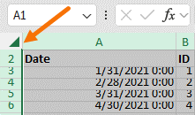
To make your data properly visible, select the whole worksheet by clicking this triangle:

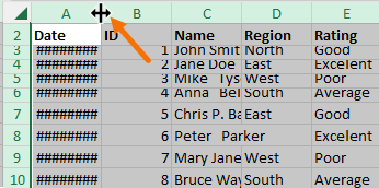
Next, bring your cursor between any 2 column labels within your dataset until it's converted into the double-headed arrow > double-click.

The same can be achieved using the keyboard shortcut CTRL+A to select the data and ALT,H,O,I to auto-fit column width.

Similarly, you can repeat the process to autofit the rows.

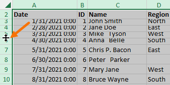
The keyboard shortcut for data auto-fitting row height is ALT,H,O,A.

While it's a quick and easy fix, it ensures that no data is overlooked. Once all your data is visible, move on to the next step.

2: Identify and Remove Duplicates

Duplicates are rarely intentional. You can use conditional formatting to highlight duplicates in your data, and then utilize the 'Remove Duplicates' feature under the Data tab to eliminate them, ensuring each row remains unique.

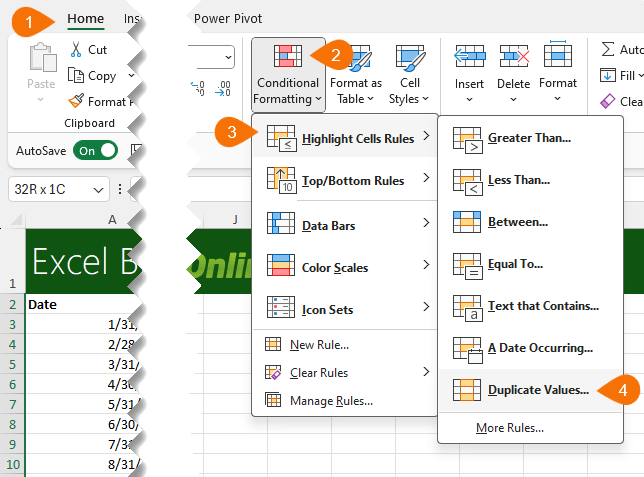
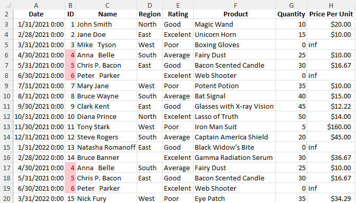
For example, in my dataset, I can quickly identify duplicates in the ID column by going to the Home tab > Conditional Formatting > Highlight Cells Rules > Duplicate values.

This opens the Duplicate Values dialog box, allowing you to choose the highlight format.

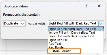
I'll go with the default settings but notice you can choose from these options or create your own custom format too.

Now I can see which rows have duplicate IDs at a glance.

I can also easily remove the duplicates, and eliminate errors from my reports.

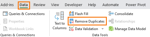
To do that, go to the 'Data' tab > 'Remove Duplicates':

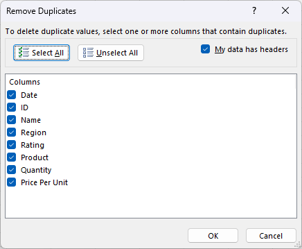
This will open the Remove Duplicates dialog box which lets us choose the columns to compare.

In this case, I want to check for duplicate rows, so I will select all the columns in my table:

And you can see Excel does the heavy lifting by deleting all the duplicate entries, ensuring each row is unique.

3: Trim Extra Spaces

Extra spaces can lead to inconsistencies. While some unwanted spaces are obvious and easy to find, others are not always visible.

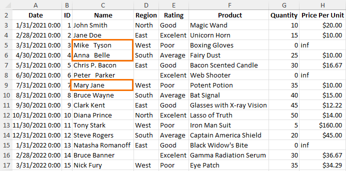
For example, the extra spaces between Mike and Tyson, Anna and Belle and Peter and Parker are easily visible however, the space in front of Mary Jane is not.

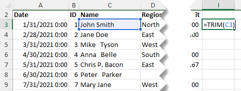
Instead of spotting and removing these one by one, it's best to employ the TRIM function in an empty column beside your data.

For example, I will use the formula TRIM(C3) in cell I3:

And then, copy it down to fix all the rows:

Once I have trimmed the data, I can copy and paste it to the original column 'as values' via the Paste dropdown > Paste Values > Values:

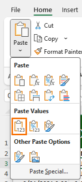
In Microsoft 365, you can also use the new keyboard shortcut CTRL+SHIFT+V to paste as values, while in older versions you can use ALT,E,S,V.

4: Eliminate Blank Cells

Blank cells can interrupt data analysis. To avoid that, you can utilize the 'Go To Special' option under the Find & Select menu to quickly select and fill blank cells, maintaining data uniformity.

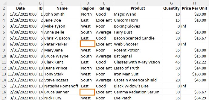
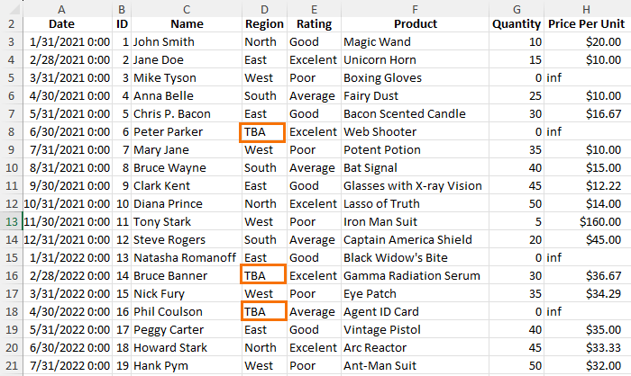
For example, some cells in my Region column are empty:

I will first select my data > Go to the 'Find & Select' menu > Select 'Go To Special':

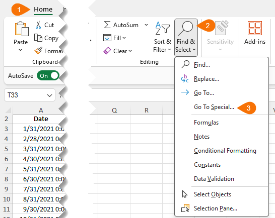
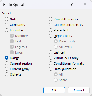
This will open the 'Go To Special' dialog box in which I need to choose 'Blanks':

And within seconds, all the blank cells in the dataset get selected:

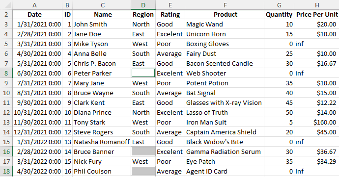
I can simply fill a placeholder value as 'TBA' in all these cells.

To do that, I can type TBA in cell D8 and then press CTRL+ENTER to enter it in all selected cells in one go.

Alternatively, if I want, I can also copy the value from the cell above.

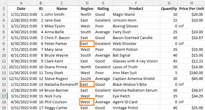
To do that, with the three empty cells selected, Type = in cell D8 > Press the up arrow > Press CTRL+ENTER.

This will fill the region of the cell above each of these blank cells, respectively.

5: Spell Check

Always run a spell check to correct typos and misspellings, a crucial step for maintaining professionalism in your reports.

For example, in my dataset, I should run a spellcheck on columns D through F, excluding the name and numeric columns.

To do that, I will select these columns > Go to the 'Review' tab > Click 'Spelling'. Alternatively, I can also use the keyboard shortcut F7.

This will open the Spelling dialog box which goes through each word in the selected cells to find spelling errors.

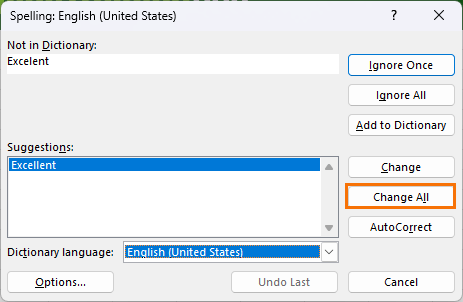
Here, it's found a spelling error in the word 'Excelent', and suggests the correct spelling 'Excellent'.

We can either ignore it or change it. It's better to change it and by clicking Change All, we ensure that any other occurrence of this misspelling is also rectified.

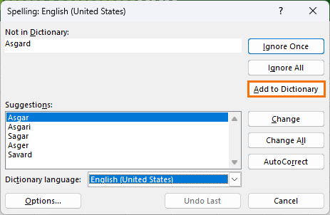
We can also select the 'Add to Dictionary' option for proper nouns such as Asgard that are not recognized English words if this is a common name we'll be using in other files.

And we're good to go!

6: Data Validation

While knowing data cleaning techniques is recommended, knowing how to prevent future errors is another skill to have in your Excel quiver.

Setting up data validation rules, like creating drop-down lists, is one of the top ways of preventing future data cleaning, as it enforces data integrity from the start.

For example, in my dataset, I can set up a dropdown list for the region column.

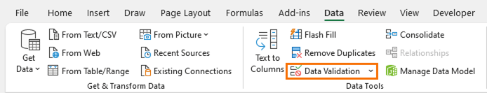
To do that, I'll select the region column > Go to the Data tab > Select Data Validation:

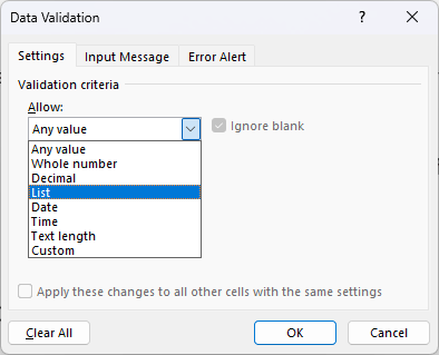
From the 'Allow' dropdown, I will select 'List':

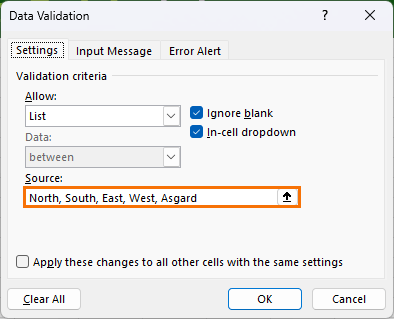
For the source, I can either reference a range of cells that contain the values, or I can just type them in with a comma separator.

I'll type in North, South, East, West, Asgard:

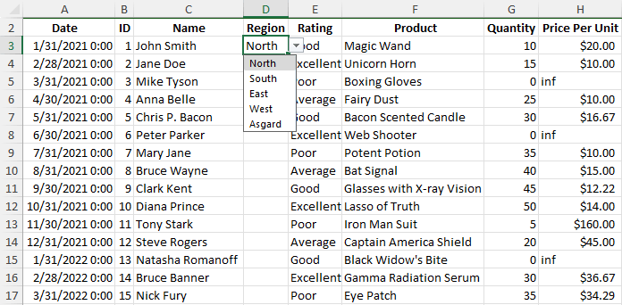
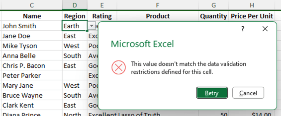
Now, whenever I will add new data, I don't need to type in the region, I can simply choose from the dropdown list:

And if I enter something not in the list, I get an error, preventing unwanted values and future data cleaning:

7: Use Tables

Another preventive data cleaning technique is using Excel tables.

Storing data in an Excel Table format can make data easier to manage, format, and analyze.

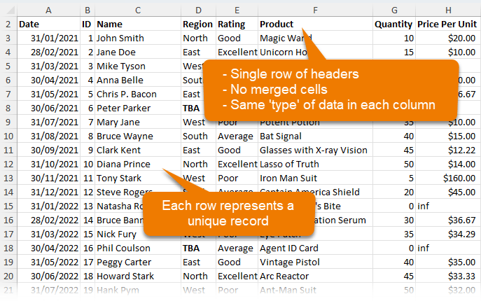
But before you can insert a table, make sure your data is in a tabular layout, and each column contains the same type of data.

In our example,

1. We have columns for the date, ID, name, region, and so on
2. Each row represents a unique record
3. Column headers are also in a single row, i.e. they're not split across multiple rows leading to merged cells.

To insert a table, use the keyboard shortcut CTRL+T. This will open the Create Table dialog box:

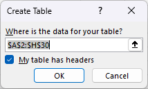
As my table has headers, I will check the box and click OK.

On inserting a table, you can instantly see the data is a lot easier to work with.

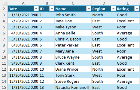
1. The headers are clearly formatted to differentiate them from the data
2. The rows are banded to allow you to easily glance across a row, which is super important in wide tables.
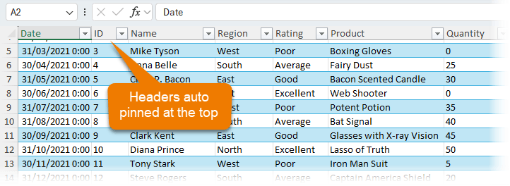
3. On scrolling down, the headers automatically pin to the top of the sheet:

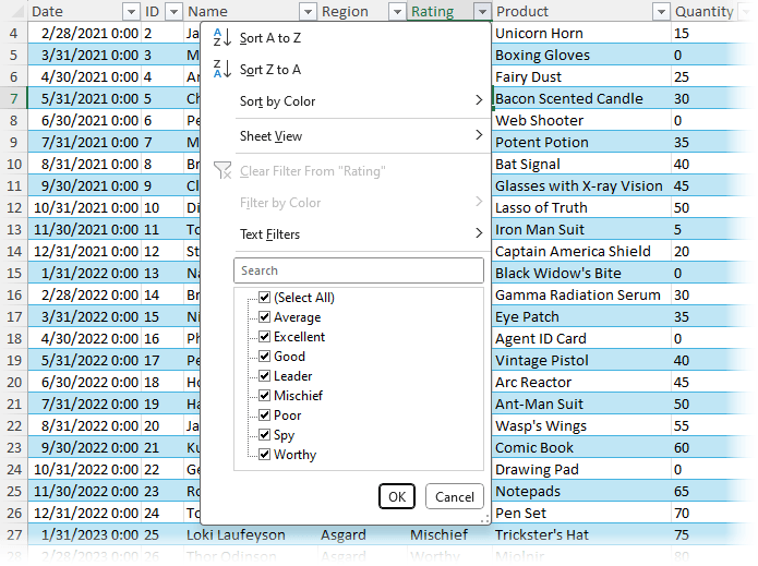
4. Each column has a filter button, allowing you to easily sort or filter your data:

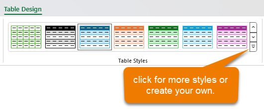
5. You can also choose from different styles on the Table Design contextual tab > Table Styles:

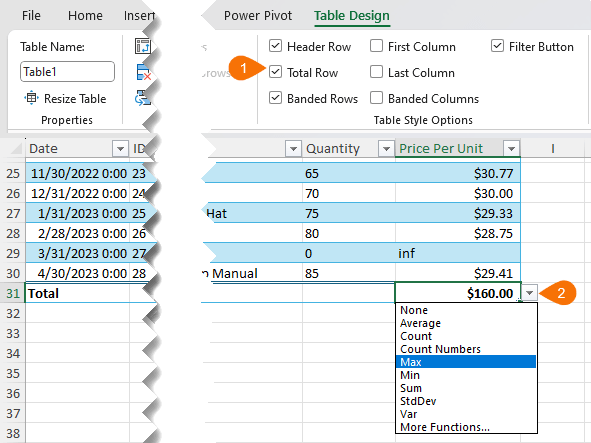
6. And, you can add a total row and change the aggregation method as required:

8: Handle Errors with IFERROR

Another great data cleaning technique involves using the IFERROR function to neatly manage and display errors in your dataset, preventing unsightly error messages from cluttering your reports.

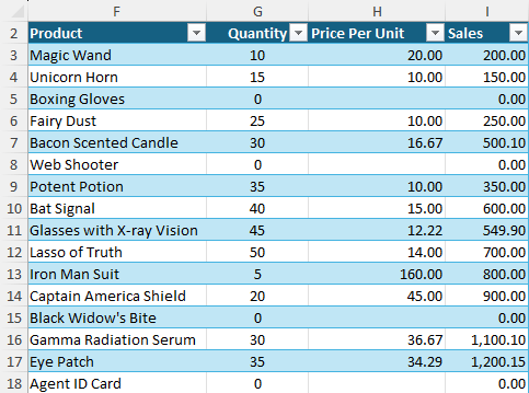
For example, let's add a column in our dataset to calculate the Sales amount by multiplying Quantity and Price per Unit.

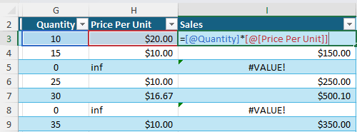
Notice the formula refers to the columns by name instead of G2*H2? These are called table structured references and Excel inserts them automatically when your data is formatted in an Excel table, and they make writing formulas super easy.

Also, when I press enter, the table copies the formula down the column for me, I don't even need to drag it down.

But wherever the price per unit is missing, the formula gives the #VALUE error.

Instead of displaying the error, we can return something else by wrapping the formula in the following IFERROR function:

=IFERROR( [@Quantity]*[@[Price Per Unit]], "Missing")

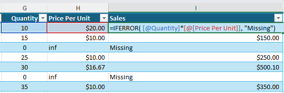
This will return 'Missing' in the rows with missing prices, instead of those ugly #VALUE errors, making your data look error-free.

Alternatively, if you don't want to mix data types in a column (which is never a good idea in your source data), you can use the below formula that returns a blank value instead of 'Missing.'

=IFERROR( [@Quantity]*[@[Price Per Unit]] , "")

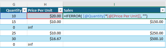
Keep in mind that you can return anything in place of an error, even another formula.

9: Number Formats

While number formats are great for presenting your data, using plain number formats during the analysis phase avoids unnecessary clutter and complexity in your dataset.

Here are the data cleaning steps for using the right number formats:

1. Use 'General' or 'Number' formats, instead of 'Currency' or 'Accounting' formats during the analysis phase
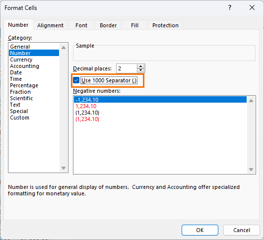
2. Always use comma separators while working with large numbers
3. Don't use the comma icon from the ribbon as it converts the number into the 'Accounting' format

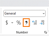
4. Instead, Open the Format Cells dialog box using the shortcut key CTRL+1 > Select Number Format > Check the box for 'Use 1000 Separator'.

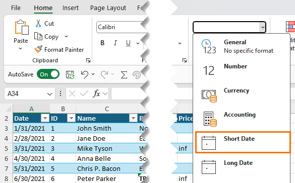
5. Also, if you have dates, format them to 'Short Date' if you don't need the time component.

10: Find & Replace

One of the most useful data cleaning techniques leverages the Find & Replace tool for bulk corrections across your dataset to maintain data consistency.

For example, in our dataset, we can replace 'inf', because as we've seen with the IFERROR example, text in a numeric column can cause problems.

To bulk replace 'inf', go to the 'Home' tab > Find and Select > Replace:

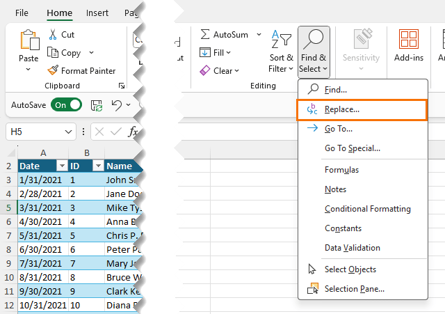
Or use the keyboard shortcut, CTRL+H.

This will open the Find and Replace Dialog box.

Here, enter 'inf' in the 'Find What' field and the value you want to replace it with in the 'Replace With' field.

I'll leave 'Replace With' blank as I want to have an empty cell.

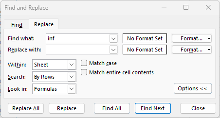
With Options expanded, notice you can also replace formats and customize where and how the Find and Replace searches the value you want to replace.

Once you've selected the desired options, click 'Replace All', and you're good to go!

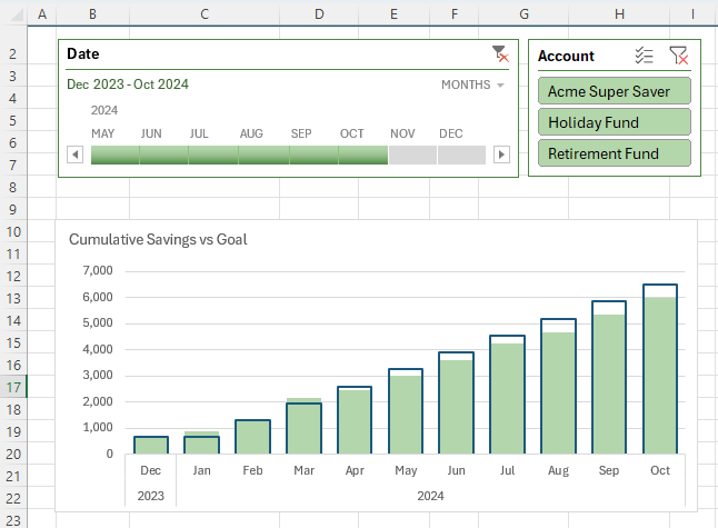
11: Remove Gridlines

Finally, if you want to present your data in a report, removing gridlines can enhance the visual clarity, making your data stand out. The report below still has the gridlines detracting from the data:

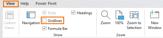
We can remove gridlines easily via the View tab > Uncheck 'Gridlines':

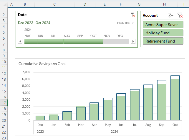
And now our report looks clean and professional:

By following these steps, you can transform a dataset into a clean, efficient, and analysis-ready format. Remember, data cleaning is not just about aesthetics, it's about ensuring the accuracy and reliability of your data analysis processes.

Next Step : Automate Data Cleaning

These techniques are great for one-off data cleaning tasks, but if you find yourself repeating these steps each week or month before you can complete your analysis or reports, then check out the video below next on how you can automate data cleaning in Excel and get updates to your data with a single click.