Excel Sorted Dynamic Unique List

I really wanted the title of this post to be “Excel Sorted Dynamic Unique List Ignoring Blanks and Errors”, but I didn’t want to brag 😉

It has never been so easy to extract a unique or distinct list of values in Excel than it is now that we have Dynamic Array formulas*.

*Dynamic Array formulas are only available in Office 365. I’ll provide links to an alternative for Excel 2019 and earlier versions at the bottom of this post.

Note: At the time of writing, Dynamic Arrays are only available in Office 365 and are currently in beta on the Insiders channel. We don’t have an ETA for when they will be available to all Office 365 users yet. And to be clear, Excel 2019 does not come with Dynamic Arrays. The only way to get them is with Office 365 …or wait until Excel 2022 (?) comes out.

Excel Sorted Dynamic Unique List Formula

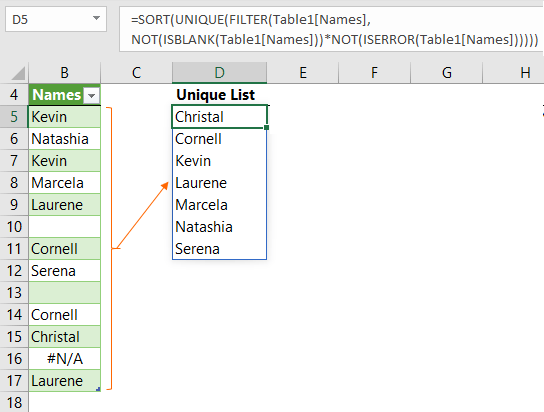
The formula for extracting a list of sorted unique values that ignore errors and blanks is super easy.

Step 1: Format the source data in an Excel Table. That way when new rows are added, or rows removed, the formula will automatically pick up the changes.

Step 2: The formula.

The most complicated part of the formula, which isn’t really that complicated, is the FILTER function, that enables us to return the list excluding errors and blank cells, among other things. The UNIQUE and SORT functions then enclose FILTER.

The FILTER function takes the following arguments:

=FILTER(array , include, [if_empty])

The array argument is the table or range of cells you want to filter.

The include argument allows you to insert a logical test specifying which values to include.

The if_empty argument is an optional value to return if there are no records that match our ‘include’ criteria. We don’t need it in this example.

The formula is:

=SORT(
UNIQUE(
FILTER(Table1[Names], NOT(ISBLANK(Table1[Names]))*NOT(ISERROR(Table1[Names])) 
    )
  )
)

In English, the FILTER formula reads:

FILTER the Names column of Table1 and return a list of values, where the Names are not blank AND the Names are not errors.

The NOT(ISBLANK(Table1[Names])) and NOT(ISERROR(Table1[Names])) formulas return a list of TRUE and FALSE Boolean values as shown below:

=SORT(
UNIQUE(
FILTER(Table1[Names],
{TRUE;TRUE;TRUE;TRUE;TRUE;FALSE;TRUE;TRUE;FALSE;TRUE;TRUE;TRUE;TRUE}*
{TRUE;TRUE;TRUE;TRUE;TRUE;TRUE;TRUE;TRUE;TRUE;TRUE;TRUE;FALSE;TRUE})
  )
)

The FALSE values are discarded before passing the list to the UNIQUE function. The UNIQUE function then removes the duplicate names before passing the list to the SORT function, which sorts it in ascending order.

If you prefer the list sorted in descending order you can add  ‘,,-1’ to the SORT formula like so:

=SORT(
UNIQUE(
FILTER(Table1[Names],
NOT(ISBLANK(Table1[Names]))*NOT(ISERROR(Table1[Names]))
  )
 ), ,-1
)

Dynamically Update

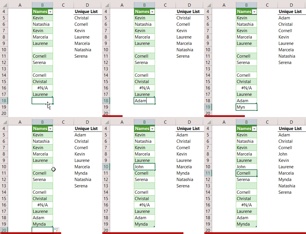
And because I formatted the source for my Excel Sorted Dynamic Unique list in an Excel Table, when I add new names it automatically updates:

Notice how the results automatically ‘spill’ to the cells below? This is the new Dynamic Array formula functionality available to Office 365 users.

Unique Lists in Earlier Versions of Excel

If you’re not fortunate enough to have Office 365 and these handy dynamic array formulas, you can use one of the techniques described here.

Related Lessons

SORT Function – there’s more to the SORT function than I’ve demonstrated here. You can also sort multiple columns and choose which column to sort by.

UNIQUE Function – the UNIQUE function can also handle multiple columns and differentiate between unique and distinct values.

FILTER Function  - you can filter more than one column and FILTER can handle OR criteria as well as AND criteria.

NOT Function – Not enables us to check if a logical test doesn’t exist.

ISBLANK Function and ISERROR Function – the IS functions check to see if a condition exists and return a TRUE FALSE, depending on the outcome. There are more IS functions at the link above.

Download the Workbook