6 Better Alternatives to the Excel IF Function

The IF function is one of the most useful functions in Excel, but it is also one of the most overused.

Because IF is so flexible, it often becomes the default solution for every type of decision, lookup, summary, or calculation. That can lead to long, complicated formulas that are hard to read, difficult to maintain, and easy to break.

For example, you might see formulas like this:

=IF(A2>=90,"A",
IF(A2>=80,"B",
IF(A2>=70,"C",
IF(A2>=60,"D",
"E"))))

This formula works, but IF is doing more than it should. In many cases, another Excel function can do the same job more clearly.

The issue is not that IF is bad. The issue is that IF is often used for jobs that other functions were designed to do better.

In this tutorial, we’ll look at six better alternatives to IF in Excel.

By the end, you’ll know when to use each one, and how to build formulas that are easier to read, easier to update, and more reliable

Watch the IF Function Alternatives Video

Get the Example File

Why You Should Avoid Overusing IF in Excel

IF is designed to test a condition and return one result if the condition is true, and another result if it is false.

A simple IF formula looks like this:

=IF(A2>=1000,"Target Met","Below Target")

This is perfectly fine.

The problems start when IF is used for everything:

=IF(D6="Unpaid","Chase Payment",
IF(E6="Out of Stock","Backorder",
IF(F6>7,"Expedite","Ship")))

Again, this formula can work. But as the number of conditions grows, the formula becomes harder to follow. You have to manage multiple opening and closing brackets, keep the logic in the right order, and make sure every possible result is covered.

In other situations, IF gets used for tasks that are not really logical tests at all. For example:

• Looking up a commission rate from a region code
• Returning a result based on a dropdown selection
• Mapping month numbers to financial quarters
• Summing rows that meet multiple conditions
• Repeating the same calculation inside a longer formula

These are all common Excel tasks, but IF is often not the best function for them.

1. Use IFS Instead of Nested IF for Multiple Conditions

The IFS function is the most obvious alternative to nested IF formulas.

It is useful when you have several conditions to test, and each condition returns a different result.

Imagine you have a list of sales orders, and each order needs a follow-up action. Some orders have not been paid. Some items are out of stock. Some deliveries will take too long. The remaining orders are ready to ship.

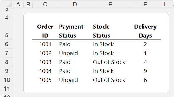
You could use a nested IF formula, but it gets harder to read as more conditions are added.

A cleaner option is IFS:

=IFS(
 D6="Unpaid","Chase Payment",
 E6="Out of Stock","Backorder",
 F6>7,"Expedite",
 TRUE,"Ship"
)

IFS works in pairs:

Excel checks the conditions in order from top to bottom. The first condition that evaluates to TRUE wins.

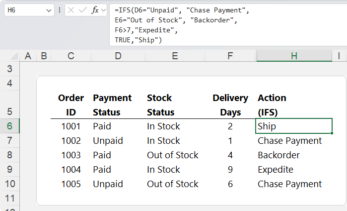
In the above example, the formula checks:

The final TRUE, "Ship" acts like a default result. It catches anything that does not match the previous conditions.

Why the Order Matters in IFS

The order of conditions is important because IFS returns the first TRUE result.

In the order status example, unpaid orders should be flagged first. There is no point expediting an order that has not been paid for.

This is why the formula checks for unpaid orders before checking stock or delivery timing.

=IFS(
 D6="Unpaid","Chase Payment",
 E6="Out of Stock","Backorder",
 F6>7,"Expedite",
 TRUE,"Ship"
)

IFS vs Nested IF

IFS is usually easier to read than nested IF because each condition and result is listed in a simple sequence.

However, there is one important difference.

IFS evaluates all conditions, even though it returns the first TRUE result. Nested IF formulas stop evaluating once they find the first TRUE result.

In very large workbooks, nested IF may sometimes be more efficient. For most everyday formulas, IFS is easier to write and maintain.

When to Use IFS

Use IFS when:

• You have several conditions to check
• Each condition returns a different result
• The order of the conditions matters
• You want a cleaner alternative to nested IF

Avoid IFS when your formula is really trying to look up a value from a table. That is a job for XLOOKUP.

2. Use XLOOKUP Instead of IF for Matching Values

A common mistake is using IF to match one value to another.

For example, suppose you have region codes, and each region has a different commission rate.

You might be tempted to write a nested IF formula that says:

• If region is N, return this rate
• If region is S, return that rate
• If region is E, return another rate

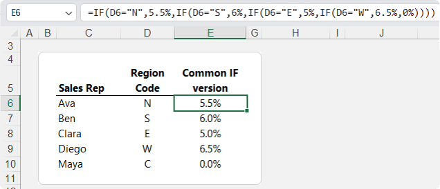
That works, but the rules are buried inside the formula. If a commission rate changes, you have to edit the formula. If a new region is added, the formula has to be rewritten.

This is not really a logic problem. It is a lookup problem.

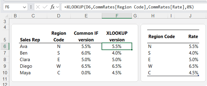
A better solution is to store the region codes and commission rates in a small lookup table, then use the XLOOKUP function:

=XLOOKUP(D6,
CommRates[Region Code],
CommRates[Rate],
0%)

Here’s what the formula does:

• D6 is the region code you want to look up.
• CommRates[Region Code] is where Excel should look for that region code.
• CommRates[Rate] is the column that contains the commission rate to return.
• 0% is the value to return if the region code is not found.

Now the commission rules are stored in a table instead of being hard-coded into the formula.

Why XLOOKUP Is Better Than IF for Lookup Tables

Using XLOOKUP makes the formula easier to maintain.

If the commission rate for South changes, you update the lookup table, not the formula.

If a new region is added, you add it to the table. If the lookup range is formatted as an Excel Table, the formula range expands automatically.

This is the key difference:

Nested IF	XLOOKUP
Tests logic inside the formula	Retrieves a matching value from a table
Harder to update	Easier to maintain
Rules are buried in the formula	Rules are visible in a lookup table
New items require formula changes	New items can be added to the table

When to Use XLOOKUP

Use XLOOKUP when:

• You are matching one value to another
• Your formula is returning a value from a table
• Your rules may change over time
• You want the formula to be easier to maintain

A simple rule is this:

If you are matching one item to another item, use a lookup table.

3. Use SWITCH Instead of IF When Testing One Value

The SWITCH function is useful when you want to test one value and return different results depending on what that value is.

For example, you might have a small report where the user chooses a metric from a dropdown list.

The dropdown might include:

• Total Sales
• Total Profit
• Profit Margin
• Average Selling Price

You could use nested IF or IFS, but you would need to keep repeating the same test:

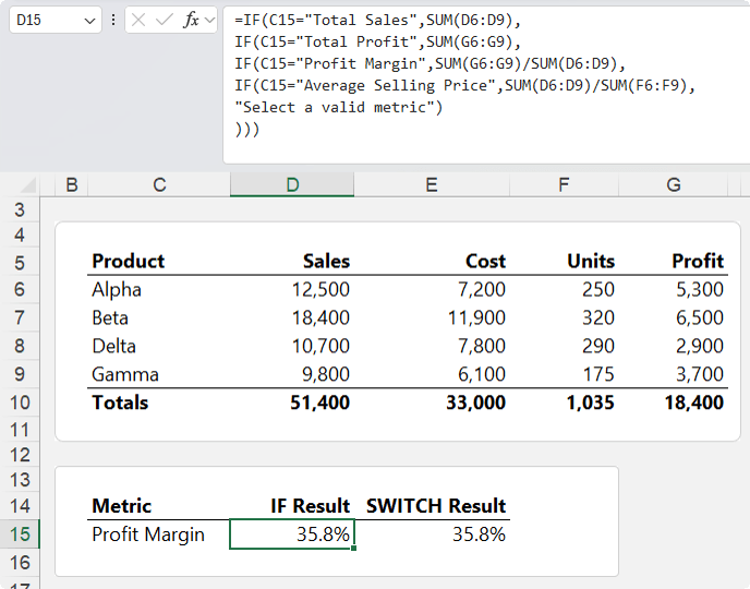
=IF(C15="Total Sales",...
IF(C15="Total Profit",...
IF(C15="Profit Margin",...
IF(C15="Average Selling Price",...

Repeating the same test is a clue that SWITCH may be cleaner.

Here is the SWITCH version:

=SWITCH(
 C15,
 "Total Sales", SUM(D6:D9),
 "Total Profit", SUM(G6:G9),
 "Profit Margin", SUM(G6:G9)/SUM(D6:D9),
 "Average Selling Price", SUM(D6:D9)/SUM(F6:F9),
 "Select a valid metric"
)

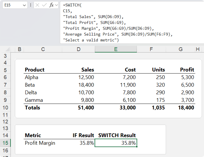
With SWITCH, you only refer to C15 once.

The first argument is the value you want to test. Then you list each possible option, followed by the result to return.

So if C15 contains:

• Total Sales, Excel returns the sum of the Sales column.
• Total Profit, Excel returns the sum of the Profit column.
• Profit Margin, Excel divides total profit by total sales.
• Average Selling Price, Excel divides total sales by units sold.

The final argument is optional, but useful. It tells Excel what to return if none of the options match.

In this case, it returns:

"Select a valid metric"

SWITCH vs XLOOKUP

SWITCH and XLOOKUP can look similar because both can return different results based on an input.

The difference is that XLOOKUP retrieves a value from a table (or reference to a range), while SWITCH can return completely different calculations.

For example, XLOOKUP is ideal for returning a commission rate from a region code.

SWITCH is better when each option needs a different formula, such as:

"Total Sales", SUM(D6:D9)

"Profit Margin", SUM(G6:G9)/SUM(D6:D9)

Each option can return a different type of calculation.

When to Use SWITCH

Use SWITCH when:

• You are testing one value
• There are several possible matches
• Each match returns a different result
• The same cell or value is repeated in a nested IF formula
• Each result may use a different calculation

SWITCH is especially useful for reports, dashboards, dropdown-driven summaries, and user-selected calculations.

4. Use CHOOSE When a Number Represents a Position

The CHOOSE function is useful when you have a number that represents a position, and you want to return something based on that position.

For example, suppose you have a month number in column D:

• January is 1
• February is 2
• March is 3
• And so on

Now suppose you want to return the financial year quarter, where the financial year starts in July.

The quarter mapping is different from a calendar year:

Month	FY Qtr.	Month	FY Qtr.	Month	FY Qtr.	Month	FY Qtr.
January	Q3	April	Q4	July	Q1	October	Q2
February	Q3	May	Q4	August	Q1	November	Q2
March	Q3	June	Q4	September	Q1	December	Q2

You could do this with nested IF, but the formula is really just mapping each month number to a quarter number:

=IF(D6<=3,"Q3",IF(D6<=6,"Q4",IF(D6<=9,"Q1","Q2")))

That makes CHOOSE a good option:

="Q"&CHOOSE(D6,3,3,3,4,4,4,1,1,1,2,2,2)

The first argument, D6, tells Excel which item to choose.

The remaining arguments are the values for positions 1 through 12.

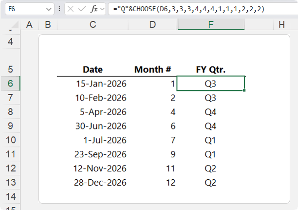
So if D6 contains:

• 1, Excel returns the first value, which is 3
• 2, Excel returns the second value, which is also 3
• 3, Excel returns the third value, again 3
• 7, Excel returns the seventh value, which is 1

Because the final result should display as Q1, Q2, Q3, or Q4, the formula adds "Q"& at the start.

So CHOOSE returns the quarter number, and the formula adds the letter Q in front.

Why CHOOSE Works Well Here

CHOOSE is a good fit because the input is already a number from 1 to 12, and each number has a specific result.

The month number acts like a position.

Instead of testing each month one by one, CHOOSE simply says:

“Take the number in D6 and return the matching item from this list.”

When to Use CHOOSE

Use CHOOSE when:

• The input is a number
• The number represents a position
• Each position maps to a known result
• You want a compact alternative to multiple IF statements

CHOOSE is useful for month mappings, scenario selections, index-based labels, and simple numbered categories.

5. Use SUMIFS and COUNTIFS Instead of IF Helper Columns

So far, the examples have returned a result for each individual row.

But sometimes you do not need a row-by-row result. You just need to answer a summary question.

For example, suppose you have the following sales table:

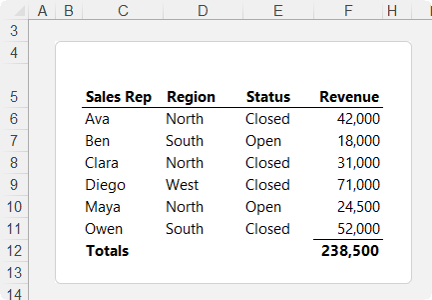
And you want to answer these questions:

1. How much revenue came from closed deals in the North region?
2. How many closed North deals are there?

A common approach is to create a helper column with IF:

=IF(AND(D6="North",E6="Closed"),F6,0)

This checks each row:

• If the region is North and the status is Closed, return the revenue.
• Otherwise, return zero.

Then you would sum the helper column:

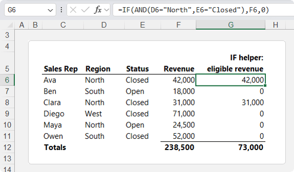
That works, but it is the long way around. You do not actually need a row-by-row result. You only need the final total.

That is exactly what SUMIFS is designed for.

Use SUMIFS to Sum Values That Meet Conditions

SUMIFS adds values that meet one or more conditions.

=SUMIFS(F6:F11,
D6:D11,"North",
E6:E11,"Closed")

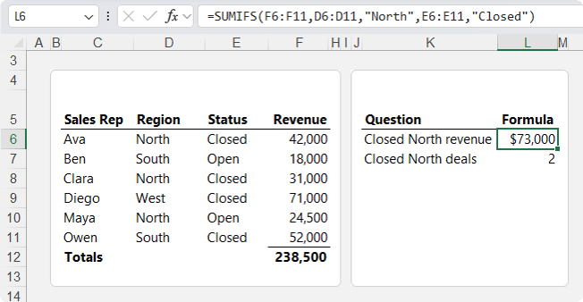
Here’s how it works:

• F6:F11 is the range to add.
• D6:D11,"North" checks whether the region is North.
• E6:E11,"Closed" checks whether the status is Closed.

The formula filters the rows and sums the matching revenue in one step.

No helper column required.

Use COUNTIFS to Count Rows That Meet Conditions

For the second question, you want to count how many closed North deals there are.

That is where COUNTIFS comes in:

=COUNTIFS(
D6:D11,"North",
E6:E11,"Closed")

COUNTIFS uses the same criteria structure as SUMIFS, but it counts matching rows instead of adding values.

In this example, it counts rows where:

• Region is North
• Status is Closed

When to Use SUMIFS and COUNTIFS

Use SUMIFS or COUNTIFS when:

• You need a single summary result
• You are applying one or more conditions
• You do not need a helper column
• You are building reports or dashboards
• You want a formula that summarises the dataset directly

These functions are especially useful for management reports, KPI dashboards, sales summaries, and financial analysis.

6. Use LET to Simplify Repeated Calculations

Sometimes the problem is not the IF function itself. The problem is that the formula repeats the same calculation multiple times.

That is where the LET function can help.

LET allows you to name part of a formula, then reuse that name later in the same formula.

This can make formulas easier to read, easier to maintain, and more efficient.

Example: Commission Based on Net Sales

Suppose you are calculating commission based on net sales.

Net sales are calculated as:

Sales less discount

The commission is only paid if net sales meet or exceed the target.

A standard IF formula might look like this:

=IF(D6*(1-E6)>=F6,D6*(1-E6)*5%,0)

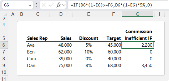
This works, but the same calculation appears twice:

D6*(1-E6)

That is the net sales calculation.

The formula uses it once to test whether the target was met, and again to calculate the commission.

In a small formula, that might not seem like a major problem. In a real workbook, repeated calculations can be longer, harder to check, and copied down thousands of rows.

Use LET to Name the Repeated Calculation

Here is the LET version:

=LET(
netSales,D6*(1-E6),
IF(netSales>=F6,netSales*5%,0))

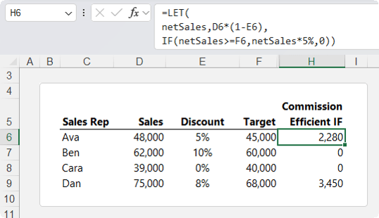
This formula creates a name called netSales.

Then it defines what netSales means:

D6*(1-E6)

Now that name can be used in the IF formula:

IF(netSales>=F6,netSales*5%,0)

The logical test becomes:

netSales>=F6

The result if TRUE becomes:

netSales*5%

And if the target was not met, the formula returns zero.

Why LET Makes Formulas Better

LET improves the formula in three ways.

First, the net sales calculation only appears once.

Second, the formula is easier to read because netSales explains what the calculation represents.

Third, if the net sales logic changes, you edit it in one place.

This is especially useful in formulas that contain repeated logic, intermediate calculations, or complex expressions.

When to Use LET

Use LET when:

• The same calculation appears more than once
• A formula is getting hard to read
• You want to name intermediate results
• You want to improve formula maintainability
• You want to reduce repeated calculations

LET does not replace IF. It works with IF and other functions to make formulas cleaner.

When Should You Still Use IF?

IF is still the right choice when you have a straightforward logical test.

For example:

=IF(B2>=1000,"Target Met","Below Target")

This is simple, clear, and easy to maintain.

IF is also useful inside other functions. For example, LET can use IF to make the final decision after defining intermediate values.

The goal is not to stop using IF altogether. The goal is to use the right function for the job.

A Practical Way to Choose the Right Function

When you are about to write an IF formula, pause and ask:

The result is cleaner formulas, fewer errors, and workbooks that are much easier to maintain.

If you enjoy learning how to build smarter formulas, check out my Advanced Excel Formulas course. It will help you move beyond memorising functions and start choosing the right formula approach for each task.

You’ll learn how to combine functions, simplify complex logic, work with dynamic arrays, troubleshoot formulas, and build more reliable Excel solutions.