Ever felt like you're spending hours on tasks in Excel that should take minutes? You're not alone.
These are my top Excel productivity tips for work and study. For each tip, I'll present a problem and a solution. Check out the video below for a demonstration.
Table of Contents
- Excel Productivity Tips Video
- Use Templates
- Navigate Using Shortcuts
- Hyperlink All Your Files
- Split, Combine, or Append Text in a Flash
- Avoid Confusing Formulas
- Get Insights Quickly
- Data Makes More Sense in Pivot Tables
- Let Excel Analyze Data for You
- Let PivotTables Do the Math
- Automate, Automate, Automate
- Next Level Productivity
Watch the Video

Download Workbook
Enter your email address below to download the sample workbook.
Use Templates
Whether it's creating invoices, project plans, or regular reports the monotony of performing these repetitive tasks each time from scratch can be mind-numbing and time-consuming.
For example, let’s say each time you have a new project start, your job is to create a new file to track progress.
You can either create a report from scratch or simply use a built-in Excel template.
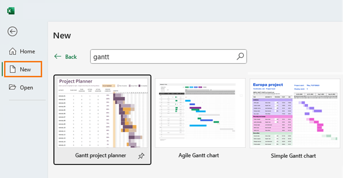
To do this in Excel, go to the File tab > New and browse for the type of template you need:
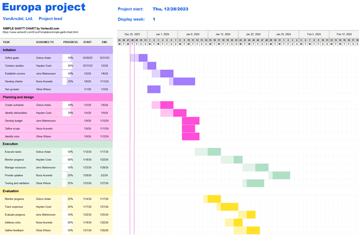
Here you can choose from a ton of built-in templates that can save you the time creating your spreadsheet. For this example, I’ve chosen the Simple Gantt chart template:
All I need to do is enter the project phases and tasks.
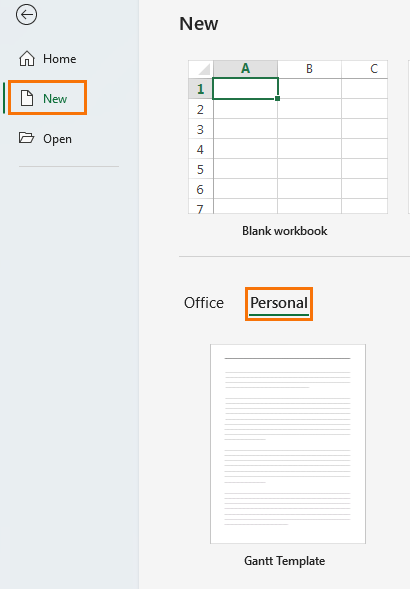
Bonus tip: If you have the same phases and tasks for each project, once you’ve made your modifications, save a copy as a template file type .xltx and it will be available in your Personal templates:
Benefits:
- Less time-consuming: You save a lot of time not having to create your spreadsheet from scratch.
- Maintains consistency: Consistent use of the same template results in efficiency gains for those who use them regularly.
Limitations:
- Needs tweaking: Built-in templates are very useful, but they often need some tweaking to suit your needs. Alternatively, you can use them to get ideas from which to create your own.
Navigate Using Shortcuts
Navigating through Excel can feel like torture, especially with large datasets. Slow navigation in Excel can significantly hamper your productivity, turning quick tasks into lengthy processes.
That’s why Excel has hundreds of keyboard shortcuts to make you feel like an Excel wizard.
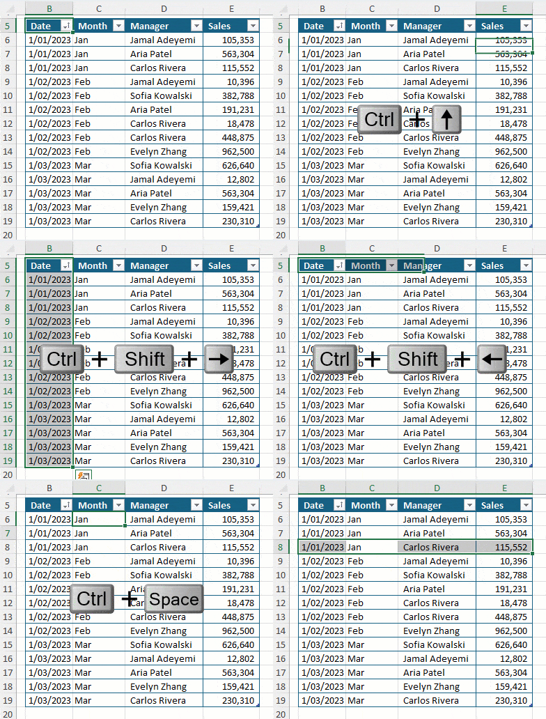
Some of the best being CTRL+ any of the arrow keys. They whisk you to the edge of your data range without needing to scroll!
For example, CTRL+Down helps you go to the end of the data range, while CTRL+Up brings you back to the top, and CTRL+Left and CTRL+Right take you in those respective directions.
Also, you can easily select a range of cells with the CTRL+Shift+Arrow Key shortcut and quickly format the cells by pressing CTRL+1. But don’t stop there – don’t even think of touching the mouse, simply navigate through the tabs using CTRL+Page Up or Down and then tab to jump through the options, then ENTER to apply one.
If your data is in an Excel table you can select a column in the table with CTRL + Space and a row with SHIFT + Space.
And of course, don’t forget your everyday essentials - CTRL+Z for undo, CTRL+C for copy, and CTRL+V for paste. And for Microsoft 365 users the new, CTRL+SHIFT+V is paste values is amazing.
Get our 239 Excel Shortcuts for Windows & Mac PDF and Period Table of Shortcuts here:
239 Excel Keyboard Shortcuts PDF and Periodic Table

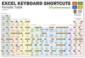
Work faster and more efficiently with our list of Excel shortcuts.
While these shortcuts are great for navigating within an Excel workbook, check out these shortcuts for navigating multiple workbooks.
Hyperlink All Your Files
When working with multiple Excel files, finding and opening the right one can be a problem and hurt your productivity, especially if they're not well-organized.
But what if you don’t need to repeatedly go back and forth into different folders within your computer to look for them?
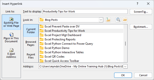
You can simply create a file map in your Excel sheet from the Insert tab > Link. Or you can learn from the last tip and use CTRL + K keyboard shortcut.
From the Insert Hyperlink dialog box, you can insert the file path in the Address field and a display name in the “Text to Display” field.
This way, not only can you add links to files on your machine, but also to your shared drives such as OneDrive, and your most frequently referred webpages.
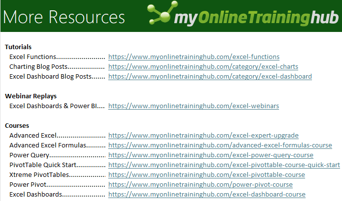
I too have created a hyperlink map with the links to all my courses, so all of you can easily find the course you want to take next.
Benefits:
- Access related files from one location: You need not search for your files every time you need to access them.
Limitations:
- Manually insert links and text: While hyperlinks are very useful, you need to manually add them and the display text which can be time-consuming but only needs to be done once.
Split, Combine, or Append Text in a Flash
Sometimes you might need to split data in one cell into two or combine two cells into one. Doing it by hand is slow and boring.
But Excel is very smart if you know how to use it to your advantage. It can recognize patterns and make your work much easier.
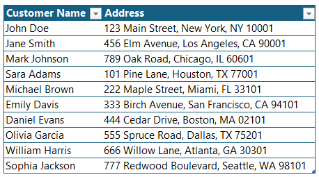
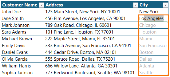
For example, let’s say I have a list of 100 Customer addresses:
I want to understand which cities and zip codes I need to send the deliveries to. For this, I need to extract the cities and zip codes into separate columns.
I can easily train Excel to do this as follows:
Add two more columns > Type the city name in the first 2 cells in the city column> Press ENTER when you see the ghosted names getting filled in automatically in the rest of the cells.
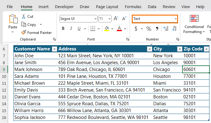
You can repeat the process for Zip Codes, but ensure that you first change the column format to Text to not lose the leading 0s
At times, if Flash Fill’s ghost values don’t show up, you can either use the keyboard shortcut CTRL + E or Go to Data > Flash Fill
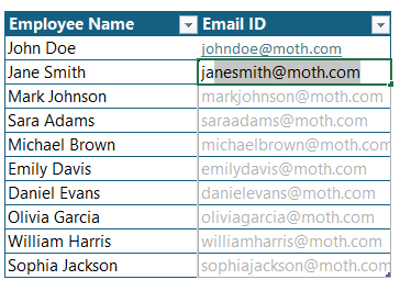
Flash Fill can also append text to your existing data also, for example, it can help you in creating Email IDs for all your employees.
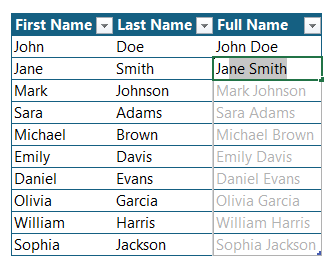
Also, it can also combine the values of two columns too.
Benefits:
- Simple to use: Flash Fill is very easy to use and can be applied by any Excel user, beginner or advanced.
Limitations:
- Requires manual triggering: Every time you need to Split, Add, or Combine data, you need to trigger Flash Fill, either from the Data Tab or using the shortcut
- Doesn’t update: If you add new data to your dataset, Flash Fill is not auto-applied
To avoid running into these limitations, or if you need to repeat such processes frequently Power Query is a much better solution. It automates the process with just the click of a button (Sometimes even that’s not required!).
Check out this simple Power Query tutorial video/blog on automating text splitting to become more productive than ever!
Avoid Confusing Formulas
Sometimes Excel formulas are hard to understand, especially if they're really long or complicated.
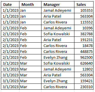
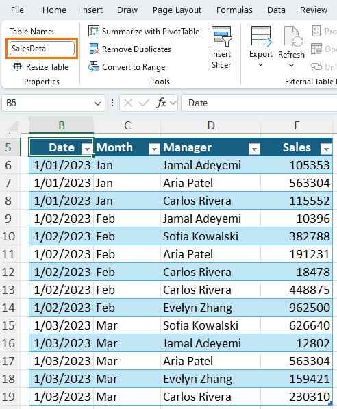
For example, here I have a dataset containing the sales of 5 managers for 3 months.
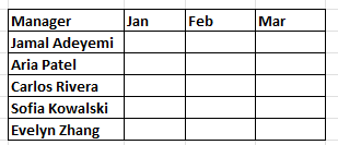
I want to create a smaller table from this dataset that gives me the monthly sales by manager. To do that, I have prepared a table as follows:
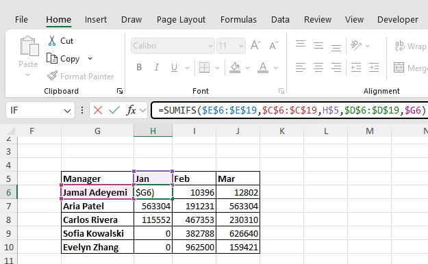
Now I want to populate it with values. I can use SUMIFS to do that with my criteria being month and manager.
I use the formula:
=SUMIFS($E$6:$E$19,$C$6:$C$19,H$5,$D$6:$D$19,$G6)
Although I get the right values, this formula looks very confusing. Without the Excel tooltips, I can’t be sure which cells refer to which values.
If I need to adjust this formula later, I will first have to understand it before I can make any changes. Also, such formulas don’t work well when you collaborate with other people on the same spreadsheet.
To avoid wasting time, it’s better to use Excel Tables and Structured References.
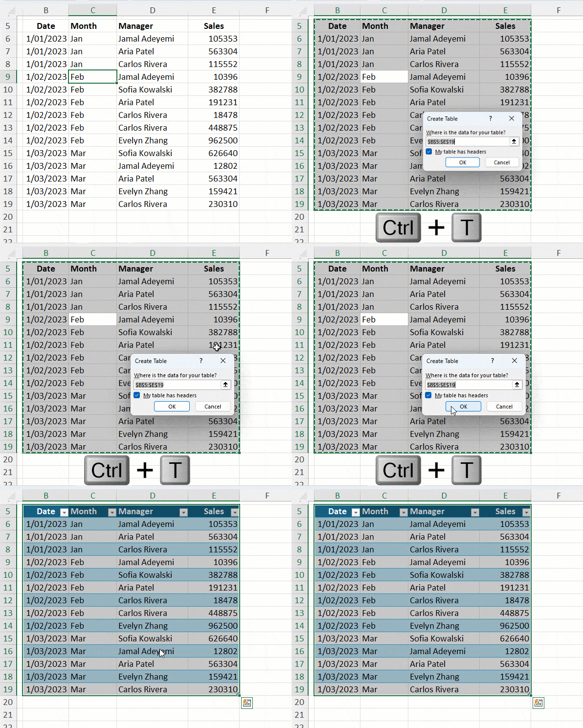
First, I need to ensure that my sales data is in a table. To do that, select any cell within my data > Press CTRL+A to select all > Press CTRL + T
Tip: if you don’t have any blank cells in your data, you can skip CTRL+A as Excel will automatically detect the outer bounds of your data.
This will insert a table around my data.
I will also rename this table to SalesData, instead of using the generic name auto-assigned by Excel.
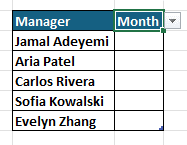
Next, insert a 2-column ManagerPerformance table with the following column headers and a few rows, one for each manager:
Select the required number of cells in the Excel gird > Press CTRL+T (I will check the “My table has headers” box)
I’ve added manager names to the rows and a Month Data Validation Dropdown to the column header.
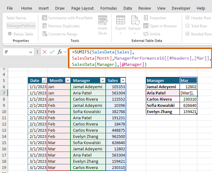
Now, to populate the total sales by manager, I will use the SUMIFS function again, but this time as my input data is in a table, I can use structured references in my formula. So, my formula looks like this:
=SUMIFS(SalesData[Sales],
SalesData[Month], ManagerPerformance[[#Headers],[Mar]],
SalesData[Manager],[@Manager])
Compared to the previous formula this formula is a lot clearer. I can discern what each component of the formula represents, they are not unnamed ranges.
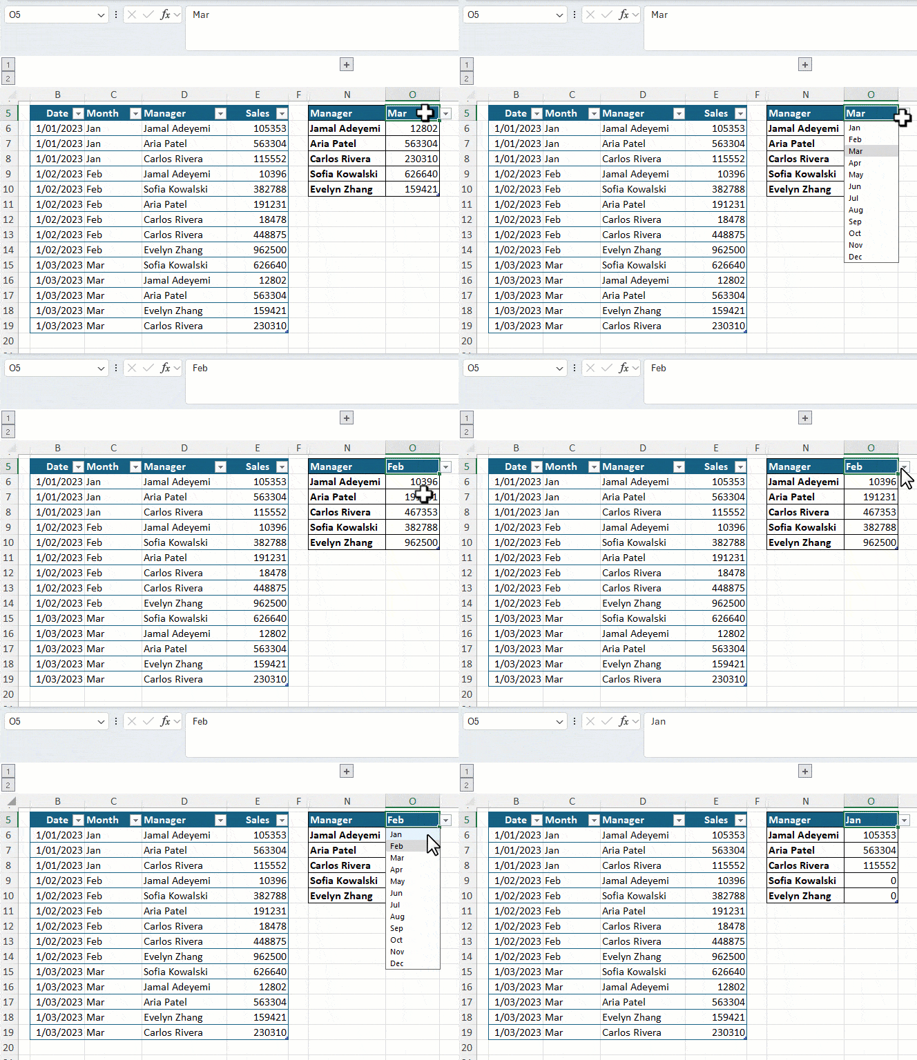
Using this formula, I get the same output as before:
Tip: This formula is dynamic because the month header is a data validation output. Therefore, if you select another month, the formula updates too!
Benefits:
- Auto updates: When I add more data to the SalesData table, the ManagementPerformance table automatically includes it.
- Less Error-Prone: Structured references make formula editing less error-prone.
Limitations:
- Incompatible with Dynamic Array Functions: Tables are incompatible with Dynamic Array Functions, so you can’t use the UNIQUE function to extract a unique list of managers from the SalesData table and populate the ManagerPerformance table.
Get Insights Quickly
Getting lost in large datasets is pretty common and it’s easy to lose sight of some important numbers.
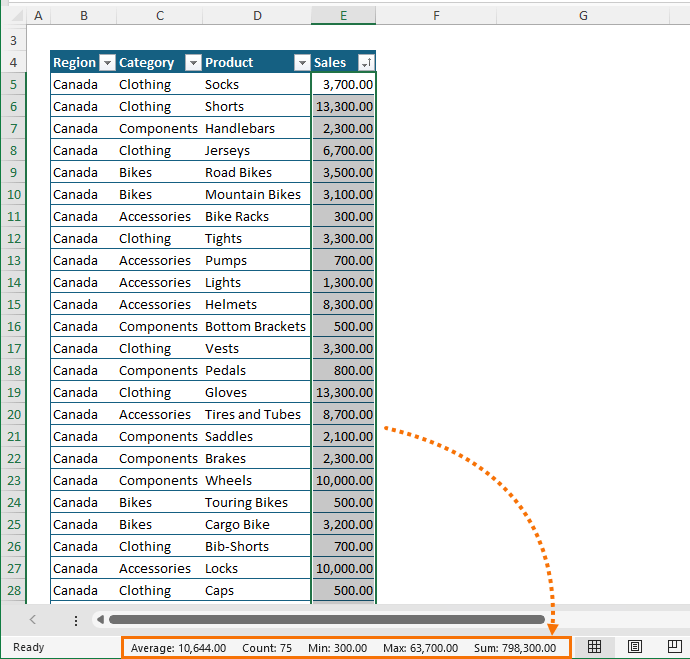
But Excel ensures you always have these numbers, if not at your fingertips, then in the status bar at the bottom of your spreadsheet.
The moment you select a column of data, like the Sales column in my dataset, you’ll notice the values such as Average, Count, Min, Max, and Sum displayed right there, in plain sight!
These come in very handy while adding, removing, or filtering data as they eliminate the need to write these formulas ourselves.
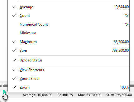
To add or remove the statistics included in the status bar, right click and then choose from the pop up menu:
Bonus tip: left click the values in the status bar to copy them.
Benefits:
- No calculation needed: These values are auto-calculated for you.
- Customizable: You can right-click on the status bar to add or remove the required values
Limitations:
- Offers basic calculations only: You can’t use this for more complex calculations, such as SUMIF or COUNTIF.
Data Makes More Sense in Pivot Tables
Ever feel like you're lost in a sea of numbers when trying to make sense of big data in Excel? It's like every cell is a puzzle piece, and you're not sure how they all fit together.
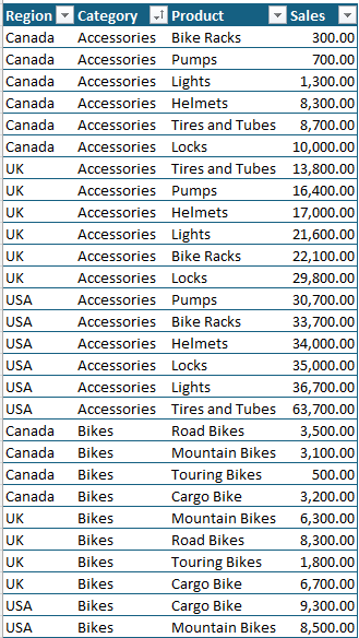
Let’s look at an example. Can you make any sense of this data?
How about now?
That’s exactly why PivotTables are a lifesaver when it comes to analyzing big data. You can break it down by country, category, product and much more within seconds!
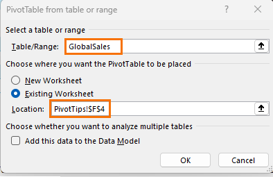
To insert a PivotTable go to any cell in your data > Insert Tab > PivotTable:
In the dialog box select where you want to insert your PivotTable. Here I have inserted it in the existing sheet, alternatively, you can insert it in a new sheet.
If you check the Add to Data Model Box, you can even access Excel’s advanced Power Pivot feature, but that’s a topic for another day.
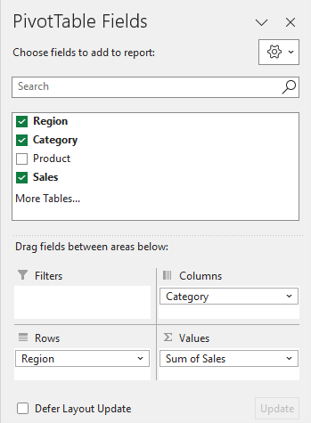
Now, simply drag the fields you want to analyze to your PivotTable, for example, here I have Region in rows, Category in columns and, Sales in values.
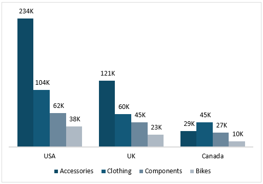
And boom! It breaks down the sales by region and product category.
You may even insert a chart to visualize your data from the Insert tab > Charts
Make sure you select a cell within your PivotTable to insert the chart.
Benefits:
- Easy to create: PivotTables are very easy to create and don’t require any formulas or coding knowledge.
- Updates include new data: When you add more data to the source data table, and refresh your PivotTable, it automatically includes the new data.
Limitations:
- No real-time updates: Pivot tables are not automatically updated in real-time. You need to refresh them manually whenever there are changes to the source data.
Let Excel Analyze Data for You
Identifying patterns and trends in data can be like finding a needle in a haystack, especially in large datasets like the one we just used.
Therefore, it’s quite possible that you might overlook crucial insights. This is where Excel’s Analyze Data feature comes in very handy.
All you have to do is Select a cell in your data > Home tab > select Analyze Data
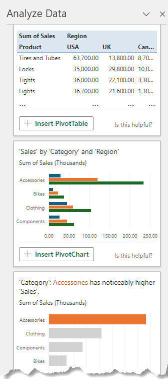
And it will identify patterns, trends, outliers, correlations and more! You can add any of the insights it returns to your report with the click of a button.
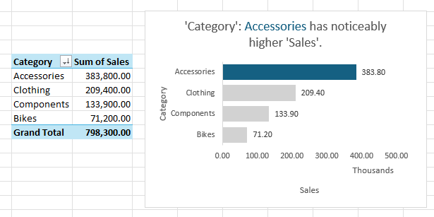
It will automatically create the PivotTable and the chart for you!
You can even use this feature to calculate important decision-making metrics such as Percentage of Sales by Product, in a jiffy!
Benefits:
- Speeds up Dashboarding: Using this feature, you can quickly create actionable dashboards.
- Identify anomalies: Analyze data scans your dataset for trends, patterns, outliers and anomalies uncovering insights you could easily miss.
Limitations:
- Needs formatting: While Analyze Data speeds up the PivotTable and chart creation process, you may still need to format them to meet your design requirements.
- Static titles: the descriptive chart titles do not update with changes to the underlying data.
Let a PivotTable Do the Math
Instead of manually writing SUMIFS and COUNTIFS formulas etc., use PivotTables to rapidly create them.
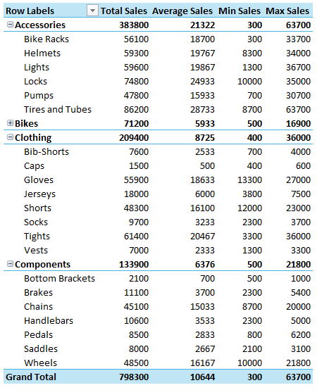
For example, you can use them to calculate total, average, min and max sales among others, using the value fields settings option.
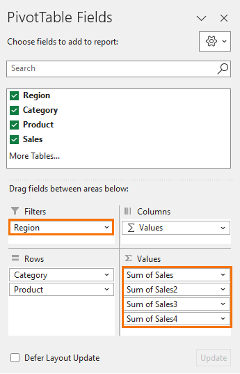
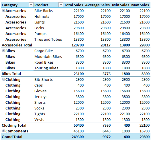
Using the same dataset, I have inserted a new PivotTable with Category and Products on Rows, and dragged sales 4 times to the values section.
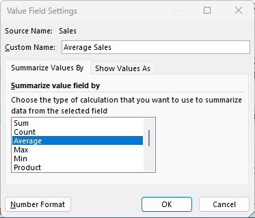
Right-click on one > Select Value Field Settings > Calculate Average Sales.
Repeat the same for Min and Max to have all 4 calculations in a single PivotTable, without even applying a single formula.
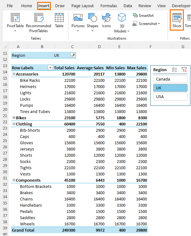
You can even add a field to the filters, for example, here I have added region to be able to see these calculations by country.
Or you can easily insert a Slicer from Insert tab > Slicers
Slicers make filtering much more intuitive.
Benefits:
- No need for formulas: PivotTables reduce the need for using formulas such as SUMIF and COUNTIF etc.
- Easy to filter: PivotTables are very easy to filter using the Slicers. Slicers also filter the associated chart.
Limitations:
- Limited calculation options: PivotTables offer only a few calculations from the Value fields settings, for more advanced calculations you can try Power Pivot.
Automate, Automate, Automate
And we are back to where we started! The most important productivity tip for Excel is to automate. Create templates, codes, or queries for everything you do repeatedly, and PivotTables are no exception.
Let’s say you have incorporated PivotTables in your routine tasks, but every time you spend a few minutes formatting them.
That sure calls for automation. PivotTables allow you to save your preferred layout as a default, so you don’t need to reinvent the wheel each time you insert one.
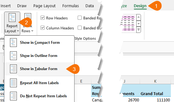
For example, instead of the default Compact format, I can choose “Show in Tabular Form” from the Design tab > Report Layout.
This eliminates the need for expanding and collapsing Category and Product on the rows.
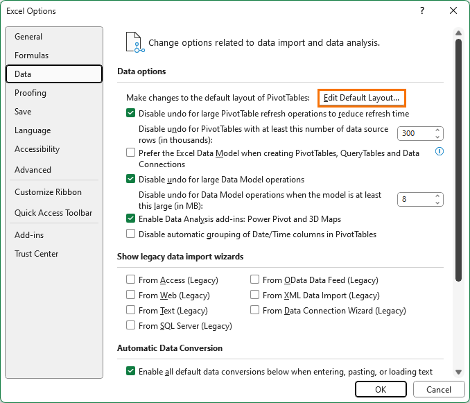
Now I can save this layout as a default from
File> Options> Data > Edit Default Layout
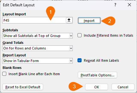
Select a cell from your PivotTable > Press Import
Or we can change values in this dialog box itself.
Now whenever you will insert a new PivotTable, it will automatically pick up this style!
I hope these top 10 productivity tips become your secret weapons to conquer Excel challenges and boost your efficiency. Try them out, and you'll be amazed by the difference they make in your work.
Next Level Productivity
Up to 80% of our time can be spent gathering and cleaning data in Excel. The ability to automate these laborious tasks with Power Query can be life changing. Don’t take my word for it, read the comment below that was left on my introduction to Power Query tutorial:
If you spend any time gathering and cleaning data, then Power Query will be a game changer for you. Get up to speed quickly with my Power Query course.







Excellent explanation for work exercises.
Thank you,
Eddie Cordero
Thanks so much, Eddie!