Wildcards *?~....what am I talking about? And no, it's not an expletive. Let’s start with an example.
COUNTIF using Wildcards

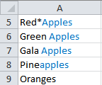
What say you wanted to count the number of cells containing the word ‘apple’ in this table.
You could simply use a wildcard (an asterisk, *, is a wildcard in Excel) in your COUNTIF formula like this:
=COUNTIF(A5:A9,"*apples*")
Your result will be 4.
Notice that the wildcard search is not case sensitive and it will count any instance of the word, even where it’s not a word on its own like in the case of ‘Pineapples’.
Alternatively, if you wanted to reference a cell instead of typing in the word ‘apples’ your formula would be:
=COUNTIF(A5:A9,"*"&A1&"*")
Where cell A1 contains the word ‘apples’.
All we are doing here is adding an asterisk to the word ‘apples’ in A1 using the ampersand. More on using the ampersand (&) to join text.
SUMIF using Wildcards
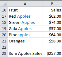
The SUMIF formula in cell B23 is:
=SUMIF(A17:A21,"*apples*",B17:B21)
VLOOKUP Formula using Wildcards
In the table below is a list of Car Manufacturers and their location. We’ve named the range of this table car_manufacturers.

In column B of the table below we want to find the location of the car manufacturer but we only want to type in the short name for the manufacturer into Column A. e.g. 'Ford' instead of 'Ford Motor Company of Australia'.
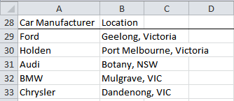
In cell B29 our VLOOKUP formula is:
=VLOOKUP("*"&A29&"*",car_manufacturers,2,FALSE)
Again, we’ve used the ampersand to add wildcards around ‘Ford’ in cell A29 before we look it up in our car_manufacturers table.
The Final Word on Wildcards
The other Wildcards you can use are the question mark ? and tilde ~.
The asterisk we've used already allows you to search for a string of text, but if you only want to search for one variable you can use the question mark wild card like this:
? Wildcard
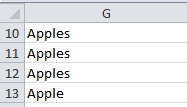
=COUNTIF(G10:G13,"apple?")
gives a result of 3.
Notice it will find words ending in 's' like 'apples' but won't find 'apple' because the ? is a place holder for another character.
~ Wildcard
=COUNTIF(A5:A9,"*~*apples*")
give a result of 1
The tilde wild card allows you to search for words that contain a wild card - either * or ?.
Simply placing the tilde before the asterisk tells Excel that the asterisk is not to be used as a wildcard.
There are other formulas you can use Wildcards with so feel free to experiment. Please post your discoveries in the comments below for all to share.
Enter your email address below to download the sample workbook.
If you liked this sign up for our Excel newsletter below and receive weekly tips & tricks like this straight to your inbox.


Very many thanks for your generosity in training us to be best in the use of Excel at zero cost.
This is awesome, thanks.
You’re welcome, Dan! Glad we can help.
Mynda,
Is there a way to print all of these without having to click – thanks!
Hi Justine,
I’m not clear on what you are trying to print?
Regards
Phil
Your solutions are very clever, please can you help with a formula to extract a registration number from mixed text in a cell that includes the rego somewhere. Here are a few examples, see list below:
The rego number is always 3 numbers & 3 letters e.g. below 332TCF
AV0386, 332TCF, 25Seater Bus, 0293, OH150325
AV0151, Hilux, 639SIW, OFA, off Hired 04/12/14
BQ93YO
(094SLP) Toyota Hilux (Avis)
(BS88ML) Toyota Hilux (avis)
LV1319, LC UTE, 159TRP, Rural, B Josephs
(368TFM) Toyota Prado
(001TGU) Mazda BT50
199VBE
865SLJ Toyota Hilux Cab (HV1256)
734TIU
(814TIZ) Mazda BT50
Thank you
Brendan
Hi Brendan,
To do that, the easiest way is to use a function, using a regular expression pattern:
Function RegCode(ByVal Text As String, Optional Pattn As String = "[0-9]{3}[a-zA-Z]{3}") As StringDim Result As String, i As Integer
Dim allMatches As Object
Dim re As Object
Set re = CreateObject("vbscript.regexp")
re.Pattern = Pattn
re.Global = True
re.IgnoreCase = False
re.MultiLine = False
Set allMatches = re.Execute(Text)
For i = 0 To allMatches.Count - 1
Result = Result & "," & allMatches.Item(i)
Next
If Len(Result) <> 0 Then
Result = Right(Result, Len(Result) - 1)
End If
RegCode = Result
End Function
Just add the above function in a vba module, and all you need to do next is to use this new function in worksheet cells, like:
=RegCode(A1) (the pattern is optional, by default the 3 digits and 3 alpha chars will be used: “[0-9]{3}[a-zA-Z]{3}” (it’s written inside the function)
You can also specify other patterns, if you like:
=RegCode(A1,"\(([a-zA-Z]{0,9})([0-9]{0,5})([a-zA-Z]{0,9})\)")I won’t tell you what this pattern does, you will have to find that yourself 🙂Cheers,
Catalin
PPPPPPPPP = 9 whose formula using
Hi Rizwan,
Sorry, I don’t know what you mean.
Mynda
Lets say I wanted to count the number of cells containing the word ‘apple’ in your table… a red apple, gala apple, macintosh apple as those are “apples”. I don’t want a pineapple because it isn’t an apple – its a pineapple. What formula would you use then?
Hi Wanda,
The first step to build a formula, is to analyze the data. Identifying patterns in data is the most important in this case. In this case, i will use this pattern: “the word apple has a space in front of it, if ‘apple’ is contained in another word, don’t count it”. For these 4 values: “red apple” , “macintosh apple” , ” gala apple”, ” pineapple”, the function: =COUNTIF(A12:A15,”* apple*”) will return 3, because “pineapple” does not correspond to the pattern. The “*” wildcard used in criteria will tell the function that there can be any characters in front of and after the sequence ” apple”.
Hope it’s clear 🙂
Catalin
Wild cards don’t work in array formulas or with SUMPRODUCT:
=SUMPRODUCT((C3:C10)*(B3:B10″Invoice $”)*(B3:B10″Ck #483″))
or
{=SUM((C3:C10)*(B3:B10″Invoice $”)*(B3:B10″Ck #483″))}
I wanted to use “Invoice*” and “Ck*” but the “wildcard” asterisk is ignored.
Hi Brad,
You can use this formula:
=SUMPRODUCT(C3:C10*(ISNUMBER(SEARCH("ck*",B3:B10))+(ISNUMBER(SEARCH("Invoice $*",B3:B10)))))Array entered i.e. CTRL+SHIFT+ENTER
Kind regards,
Mynda.
Mynda,
I can’t find anything that states this outright but it seems that the wildcards will not include empty strings. So if I do a SUMIFS statement and the values for one of the conditions are NULL or a blank string, it will not include those corresponding values in the sum. Is there a work around that you know of?
Example referencing your SUMIF statement above: if you change the formula to =SUMIF(A17:A21,”*”,B17:B21) and delete the “green apples” in A18, the result is $241.00.
Hi Angelique
You can use this SUMPRODUCT formula:
Kind regards,
Mynda.
from iran
thanks of help
You’re welcome 🙂
Thank you very much for your website; it’s wonderful finding _clear_ answers to my Excel questions.
You’re welcome, Michael 🙂
Just for your information:
This formula works beautifully with sumif also.
=SUMIF(A5:A9,”*apples*”)
Rgds,
Subash
Hi Subash,
Thanks for sharing.
Carloe
ps: I got your file already from HELP DESK. I’ll send it to you ASAP.
Just wanted to say thank you. Your website was very helpful
Hi Jane,
On behalf of Mynda and Philip, You’re welcome.
Cheers.
CarloE
Your vLookup wildcard trick does not work is Column A’s keyword has multiple keywords in it. For example instead of just having “ford” if it has “ford motor” it error’s out.
Any solution for that bug?
Hi Bob,
It’s not a bug, the formula is doing what it is supposed to do. i.e. Find a specific word within a cell. It actually does work for ‘Ford Motor’ but it would give an error if you looked up ‘Ford Car’, since the string ‘Ford Car’ does not exist in the Lookup Table.
Are you saying you want to look up ‘Ford Car’ and if it finds ‘Ford’ or ‘Car’ it should give you the result? Can you please be more specific about what you want your formula to do.
Thanks,
Mynda.
I have a request similar to bob’s – I believe. I want a Lookup table that contains wildcards (e.g. *Ford*, *Audi*) and then if the string being looked up contains a match, return the value in the second column. For example, I want “Ford Car” and “Henry Ford” to return Geelong, Victoria.
Is this possible? Any assistance would be fantastic!
Regards,
Scott
Hi Scott,
I have downloaded the workbook and it works just fine.
I even tried to use ‘Motor’ as the look-up value and it still work.
I’m referring to this formula:
=VLOOKUP("*"&A29&"*",car_manufacturers,2,FALSE)and this table
Cheers,
CarloE
please show me how excel formula and function is used in banking back office job. and data entry job with example
Hi Sathi,
There isn’t one, or even a bunch of formulas that are specific to ‘banking back office jobs’. I know because I worked in the back office of investment banks for 8 years. For this type of job you’d need to know Excel to an advanced level.
You can find an index of tutorials on common formulas here.
I hope this points you in the right direction.
All the best,
Mynda.
For COUNTIF using WILDCARDS, I needed a “&” before AND after the A1
so instead of
=COUNTIF(A5:A9,”*”&A1”*”) Where cell A1 contains the word ‘apples’.
use
=COUNTIF(A5:A9,”*”&A1&”*”) Where cell A1 contains the word ‘apples’.
This particular use was hard for me to find online. Thanks!
Hi Sue-Ting,
Yes, correct. You need an ampersand before and after the A1 reference. I will correct the typo in the post above. Sorry for the confusion.
Kind regards,
Mynda.
Mynda,
Your site was the only site I found that demonstrated how to do a HLOOKUP wildcard search linked to a cell reference (“*”&K3&”*”). Most have the actual value hardcoded in the formula which wasn’t practical for my purpose.
Thank you for solving my problem.
🙂 thanks, David. Glad to help out.
I am trying to use a wildcard in my VLOOKUP formula that will find values in column A that contains a value from K3 (an approximate match). If it finds K3 then I want it to sum up columns 3 through 9. Here’s what I have, which is giving me a result of 0. It should give me $65k.
=SUM(VLOOKUP(“*”&K3&”*”,A:I,{3,4,5,6,7,8,9},FALSE))
K3 = Health Care
Column A has “Health Care – Facility B”
Hi Laura,
Try typing the double quotes in Excel again. Notice how the double quotes in your formula are on a slant? When I copied your formula into Excel it didn’t work either. Then I typed the double quotes in again and voila, all good.
Oh, and this is an array formula so you’re entering it with CTRL+SHIFT+ENTER aren’t you?
I hope that fixes it at your end too. Let me know if not.
Kind regards,
Mynda.