Calculating time in Excel can be very frustrating, especially when all you want to do is sum a column of times to get the total, but for some reason you end up with a random number like in the example below.

Let me explain what’s going on and how to calculate time in Excel.
Since time is a concept rather than a mathematical equation, Excel has come up with systems for handling dates and times whereby they are given a numerical value.
Free eBook - Working with Date & Time in Excel
Everything you need to know about Date and Time in Excel contained in this free eBook and Excel file with detailed instructions.
Enter your email address below to download the comprehensive Excel workbook and PDF.

Download the Excel Workbook and PDF. Note: This is a zip file including an Excel workbook with detailed instructions and a PDF version for your reference.
Download the Excel workbook and follow along. This workbook contains the examples used in this post.
Want More Time?
Learn more about how Excel handles dates and time in our comprehensive guide to working with Excel Date and Time
Dates in Excel
Excel gives each date a numeric value starting at 1st January 1900.
1st January 1900 has a numeric value of 1, 2nd January 1900 has a numeric value of 2 and so on... These are called ‘serial values’, and they enable the use of dates in calculations.
Times in Excel
Times are seen as decimal fractions. 1 being the time for 24:00 or 0:00. 12:00 has a value of 0.50 because it is half of 24 hours, or the whole number 1, and so on.
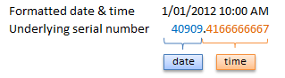
To see Excel's value for a date or time, simply format the cell as general.
For example the date and time of 1st January 2012 10:00:00 AM has a true value of 40909.4166666667
40909 being the serial value representing the date 1st January 2012, and .4166666667 being the decimal value for the time 10.00AM and 00 seconds.
Although the above is important to know, thankfully Excel has built in formatting so that we don’t have to enter our dates and times in serial or decimal values.
However it’s the lack of understanding of these serial and decimal values for time that cause common errors when performing calculations on time.
The Secret to Calculating Time in Excel
If you want to sum time (as in my example above) you need a custom format that uses [ square brackets ] around the hours. Like this:

You can see in the Sample box the correct total appears. This way I know I’ve formatted my time correctly.
These square brackets instruct Excel to add the hours. Without them it will reset the sum to zero every time it gets to 24 hours.
There’s no need to modify the formatting of the minutes with square brackets as they automatically add up.
Note: in some versions of Excel when you insert a formula it will automatically apply the correct formatting to give you the total. Just be sure to check the total is reasonable or check the formatting is as stated above.
This square bracket time formatting requirement also applies when using other operators like +/-.
What if you want to sum seconds to find out the total seconds?

While this isn’t the wrong answer, I want to know the total number of seconds, not how many minutes and seconds there are. To do this you’d need a custom number format like this:

You can see from the sample box I now get 237 seconds, instead of 3 minutes 57 seconds.
This can also be applied to minutes or hours. Just change the formatting to [mm] or [h] respectively.
Time x rate to calculate wages or charge out fees
I quite often want to calculate wages or a charge out fee. But if you don’t know this trick you’ll be tearing your hair out...and probably revert to using fractions like 7.50 for 7 hours 30 minutes, just so you can get the answer you expect.
While entering halves or quarters of an hour as fractions is fine as, it becomes a hassle when your billing increments come down to 10 minutes or any other fraction you can’t calculate in your head....unless you’re superhuman!
Thankfully the solution is simple. Just multiply by 24 like I have in the example below.

Timesheets to Calculate Time Worked
Below is a fairly basic timesheet layout. You can see in the formula bar that the time calculation is performed as a simple equation =I4-I2-I3.

I’ve done some custom formatting to the cells to assist the person keying in the time:
- Rows 2 and 4 are formatted with h:mm AM/PM. The employee has to type in their time as you see it in the cell for the formatting to work correctly. The advantage to this is they don’t need to convert their finish time to a 24 hour clock style. The disadvantage is a bit more typing with the need for the AM or PM distinction. Swings and roundabouts.
- Rows 3 is formatted with h:mm "h:mm". This adds the text h:mm to the end of the value for presentation purposes. The employee only needs to type in 0:30 for a half hour lunch break, and Excel will add the h:mm to the end.
- Row 5 is formatted with [h]:mm "h:mm" to ensure the hours are added correctly.
You can then calculate wages using the total figure in cell N5 with the Time x Rate formula above. Of course this doesn’t take into account overtime and penalty rates. That lesson is for another day.
Calculating Time that Spans 2 Days
When your start and finish times are on different dates, as in the case of shift workers, you either need to enter the Date and Time in your timesheets, or if you only enter the time then you need a clever formula to detect this. In the example below the finish time for Monday is actually 7AM on Tuesday.
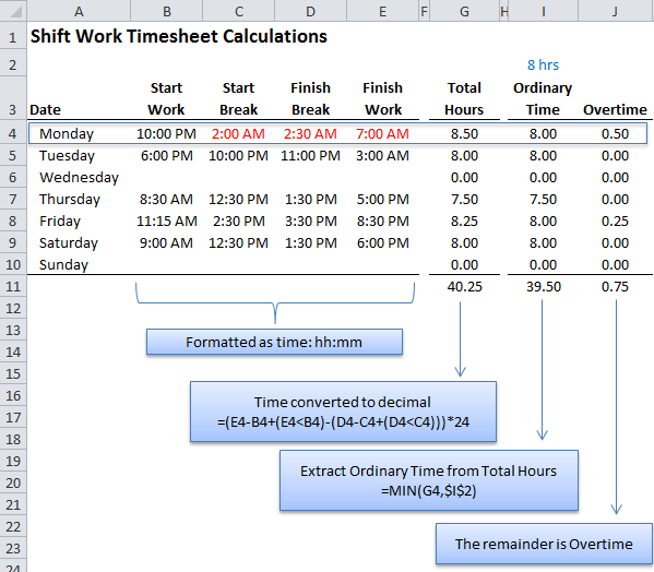
Here we can use a clever trick to test for time that finishes on a different date by checking whether the finish time is less than the start time, as is the case for Monday and Tuesday above.
Taking the formula in cell G4:
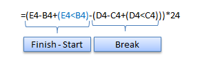
The first part of the formula takes the finish time less the start time and then checks whether the finish time is less than the start time (E4<B4).
In the case of Monday (E4<B4) evaluates to TRUE, and since TRUE = 1 it adds 1 to E4-B4 to correctly calculate the time.
Alternatively you could use a MOD formula in cell G4, like this:
=(MOD(E4-B4,1)-MOD(D4-C4,1))*24
The MOD function returns the remainder after a number is divided by a divisor.
The formula is clever because it handles negative times, which usually return pound errors, by converting them to the balance of a day (hence the 1 in the formula).
This returns the same result as the first formula [ =(E4-B4+(E4<B4)-(D4-C4+(D4<C4)))*24 ] above.
While I think the MOD function example above is super clever, it's much more difficult to explain, and more difficult to understand for those who might later inherit your spreadsheet.
Feel free to use the formula you're most comfortable with, as they both return the same result.
Note: if your times are entered with the date and time you can simply subtract one from the other, it’s only in the case where times are entered on their own that you need to test whether the finish time is < the start time.
Do you need help with a time calculation? Post your question on our Excel Forum and we'll be happy to help you.


Thank you for sharing this information about calculating time in excel.
Glad it’s useful, Elvira!
Great point! Excel’s built-in formatting definitely makes things easier, but it’s crucial to understand how serial and decimal values work with time to avoid mistakes in calculations. A little knowledge can go a long way in preventing errors!
I’m working on a worksheet to compute the total duration by adding drive time to the elapsed time between “Time In” and “Time Out.” For example, if the “Time In” is 6:00 AM and the “Time Out” is 11:00 AM, and then you have another interval from 12:00 PM to 3:00 PM, plus a 1 hour and 15 minutes drive time, I need to calculate the total number of hours.
Please post your question on our Excel forum where you can also upload a sample file and we can help you further.
Great One.
Thank you for sharing this informative information it can use in a daily work.
Our pleasure, Priya!
Sure, I’d be happy to help with the time calculations, especially considering the frequent breaks taken by the employees. It’s crucial to accurately account for working hours to ensure fairness and compliance with labor regulations.
Hi Mynda, i try to doing a time sheet using excel but i not sure how to make the calculation. below is working time.
my question is how to calculate it in excel (7.35am arrive to work, out for lunch on 12.20pm, back to lunch 1.25pm, and back on 5.05pm)
7.35am have to be counted 8.00am then 1.25pm have to counted as 1.30pm
only out time can be counted extra earn time
In Time – 8.00am
Out Break – 12.00pm
In Break – 1.30pm
Out Time – 5.00pm
Monday to Friday 8.00am – 5.00pm
Lunch time 12.00pm – 1.30pm
Saturday 8.00am – 12.00pm
Hi Nomie,
Please post your question on our Excel forum where you can also upload a sample file and we can help you further.
Mynda
Hi,
All my hour are 24 formats.
11:30 – 3:00 = 8.30 (must give 2:30)
On Excel (O8-P7 / Like to say 11:30 PM—3:00 AM)
I do not want AM/PM format.
Thanks for sharing.
If you don’t want to use AM/PM then you must enter your times in 24 hour format, so 3:00 PM would be 15:00. Note: your formula would also have to be 15:00 – 11:30 = 3:30 as you cannot have negative time in Excel.
Mynda
Hi.
How to make sum of hours and minutes for school where one hour is 45 minutes, not 60.
That means:
1 hour and 30 minutes + 1 hour and 30 minutes = 3 hours and 15 minutes
0 hours and 30 minutes + 0 hours and 15 minutes = 1 hour and 0 minutes
Thanks.
Hi Ivica,
If 45 minutes is the equivalent of an hour, then 1 hour and 30 minutes + 1 hour and 30 minutes = 4 hours, not 3 hrs 15 minutes. In which case you can divide the sum of your times 0.75 to get the equivalent 45 minute long hours. e.g. =TIME(3,0,0)/0.75 returns 4 hours.
Mynda
Hi,
I need an excel formula for calculating charges as per the time taken.
eg. For 30 minutes or less the charge will be 500 $, for every additional 30 minutes 500$ will be charged.
Please post your question on our Excel forum where you can also upload a sample file and we can help you further.
Hello, my question is on calculating elapsed time over a period of days.
I need help with the proper formula to calculate elapsed days, hours, minutes. I keep track of certain projects and need to calculate how long it took each individual to complete it, we work on an 8 hour schedule Mon-Fri sometimes Saturdays. I have a start date and time also, end date and time. I need to figure out how long it took for this piece to be completed during working hours. Current formula I’m using gives me days, hours, minutes but does not exclude weekends.
Your help is greatly appreciated.
thank you.
Hi Olga, please post your question on our Excel forum where you can also upload a sample file and we can help you further.
Hi, hope you would know the answer. this is a puzzle for me, 0930 (or any time string with 30) will become 09:18 when use the method of divide by 2400. all other time string convert properly…..I know how to work around it, but it will takes some extra formula/column to do this which is not ideal, so I just want to know anyone has any idea why this happen and how to overcome it. I could not properly google out the right topic. Thanks
Hi Mii,
It sounds like your time are entered as decimals with 9.3 representing 9:30 when it should be 9.5 i.e. .5 of an hour is 30 minutes. In that case you can use this formula where cell A3 contains your time:
=(INT(A3)+(A3-INT(A3))/0.6)/24
If you’re still stuck please post your question on our Excel forum where you can also upload a sample file and we can help you further.
Mynda
I am completing 1 file in 30 seconds then how much time will I take to complete 10 files
What’s the formula for this calculation
Hi Divya,
You can use this formula: =TIME(0,0,30)*10
Mynda
=(F17-C17+(F17<C17)-(E17-D17+(E17<D17))*24)
please above formula for automated calculator "TOTAL HOURS", how to do that?
Date Time in BkTime out BkTime in Time out total Houre stand Houre
26-Jan-2019 Sat 12:20pm 13:00 13:10 18:00pm
27-Jan-2019 Sun 12:00pm 20:00 20:30 03:00am
02-Feb-2020 Sun
l want do learning Excel Time sheet & dble ot & nomal ot calculate.
thanks.
best regrd's
Michal Chaminda Dissanayaka.
L.E.:
Date /Time in /BkTime out/ BkTime in /Time out /total Houre /stand Houre/
.
below details for your reference, ( sent my comments)
Hi Michal,
Please prepare a sample file with your data and your expected results on our forum, it’s the easiest and faster way to provide a functional solution.
Thank you
Catalin
I need your help as I don’t know the equation to calculate the exact time for below example.
Project started on Project Ended on Exact time
02-10-19 10:00 16-10-19 13:00
Note: They take a day off (Friday) and their working hours from 9 AM to 5 PM.
Hi,
Please upload on our forum a file with sample data and expected results, including clear descriptions of how the calculation should be done.
It will be much easier to help you.
Catalin
hi sir ,
i have day shift time sheet like this time in 6.00 out 19.30 , i used formula including lunch time =((19.30-6.00)-9) answers is 4.30 OT , 9 meaning lunch 1hrs and company 8hrs , then i want night shift formula time in 18.30 out 8.00am how to minus 9hrs one shoot , i want direct over time , please can you tell me this formula. please can you email me .
Hi,
This is explained in the section headed Calculating Time that Spans 2 Days
If you are not entering the start and end dates then you need to calculate if the end time is less than the start time, and if it is then add 1 after subtracting the start time from the end time:
im trying too find out if i had 4 30minutes starting at wensday 205 PM would i end up at friday
Hi Parker,
Sorry I don’t understand your question, there’s not enough information. 4 x 30min = 2hrs so 2hrs from 2.05pm is 4.05pm???
Please start a topic on the forum and try to explain this again, and attach a workbook if you have one.
Thanks
Phil
hi i am tring to do a Tip out Time formula, Tips are 56.75 divide by 48 hours everyone work x invidual hours
Pooled tips between all servers = $500
Server A works 8 hours
Server B works 6 hours
Server C works 4 hours
Total Hours of all servers = 18
A’s tip = (500/18) X8 = 222
B’s tip = (500/18) X6 = 166
C’s tip = (500/18) X4 = 11
and if the hours/ tips change to round them down to the near cent to split efenly
Hi Paul,
This is a simple formula, but it depends on how your data is entered in the worksheet. Please post your question and sample Excel file on our forum where we can help you with a specific answer.
Mynda
Hello!
I am trying to create a simple clock out calculator (simpler said than done for me).
I want to input my Clock In (start time), Clock Out (lunch), Clock In (end lunch), and then have my Clock Out time be calculated when total hours should equal 8.
I am a novice Excel user, so finding anything about building this has been difficult!
Hi Roro,
Take a look at this file, maybe it helps: OneDrive
You can search this page for OneDrive, there are multiple downloadable samples used in comments that should help.
Regards,
Catalin
i have a finish time and date that i use to dictate the start of our production however i cannot get the finish time to work within the working hours of the day for example,
job1 finishes at 7:15 am and that will transpose to the start time of job 2,
however the start time for job 2 isnt until 08:00am
A1 = finish of job 1
B1 = start of job 2
C1 + C2 = start time + finish time of job 2s working day
could you advise how i would get this finish time if it is before the start of the next job to round up to the beginning of the working day.
Hi Joe,
You could use MAX to return 8 AM if the finish time is before 8 AM. e.g.
=MAX(cell containing the actual end time, TIME(8,0,0))
Mynda
Good I love math
How do I create a formula to reflect working 12 hrs on a given day, of work off 72 and then back working 12 : trying to create a work schedule
Hi Roseann,
Can you provide a sample file? Not easy to see what you mean without a file. You can upload it on our forum, create a new topic after sign-up.
Catalin
Good.
Hello, I have a question that may be a little difficult to explain. I am using times in an advanced filer to show instances when an event occurs on a given shift.
The issue comes into play when a shift goes from 11pm to 7am. I am using times of start and stop in separate cells with one containing >=xx:xx:xx and the other containing =23:00:00 and have values show, but when I also use <07:00:00 the filter removes times that it shouldn't.
Is there a way to look between times that span from evening to morning?
***and the other containing =23:00:00 the values show in the list, but when I also use <07:00:00 the filter removes times that it shouldn't.
Sorry, it cut off my question incorrectly.
Hi John,
Can you provide a sample file? You can upload it on our forum (create a new topic after sign-in)
It will be easier to help you.
Catalin
Hi,
I need a solution for excel sheet I am maintaining to track activities on issues I get from client.
Working hours are 09.00 am to 05.00 pm and every issue has 4 hours of time to get it acknowledged for the first time. For every issue creating after 05.00 pm (today) till 09.00 am(next day) must calculate acknowledge time from 09.00 am.
How can we do this?
Thank you,
Ankita
Hi Ankita,
Can you please upload on our forum a sample file with your calculations? Create a new topic after sign-in, it will be easier to help you with a real data set.
Catalin
Hi, I need help to fix the formula for billable time. It’s not exactly where I want it to be…
=IF(A3-B3<=TIME(0,2,0),0.1,ROUND((A3-B3)*24,1))
A3-B3 = the time difference
I am trying to fix the error when 1-8 minutes to show 0.1 of hours. In other words,
1-8 = 0.1
9-14= 0.2
15-20= 0.3
21-26= 0.4
27-32= 0.5
33-38= 0.6
39-44= 0.7
45-50= 0.8
51-56= 0.9
57 and up= 1.0
I also have this part of the formula which basically is that above, not sure how to use it
=IF(AND(1 <=X72-W72,X72-W72<=8),0.1,0)+IF(AND(9 <=X72-W72,X72-W72<=14),0.2,0)+IF(AND(15 <=X72-W72,X72-W72<=20), 0.3,0)+IF(AND(21 <=X72-W72,X72-W72<=26),0.4,0)+IF(AND(27 <=X72-W72,X72-W72<=32), 0.5,0)+IF(AND(33 <=X72-W72,X72-W72<=38),0.6,0)+IF(AND(39 <=X72-W72,X72-W72<=44), 0.7,0)+IF(AND(45 <=X72-W72,X72-W72<=50),0.8,0)+IF(AND(51 <=X72-W72,X72-W72<=56), 0.9,0)+IF(AND(57 <=X72-W72,X72-W72<=59), 1,0)
Thank you so much.
Hi Nicholas,
You can try this formula:
=INDEX({0.1,0.2,0.3,0.4,0.5,0.6,0.7,0.8,0.9,1},MATCH(A3-B3,{0,8,14,20,26,32,38,44,50,56},1))
Catalin
If I go to work at 3:30 pm and I end work in 4 hours what time do I leave
Hi Taysha,
In cell A1 enter 15:30 and in cell A2 enter 4:00. In cell A3 enter this formula =A1+A2
Mynda
okay, I’ve tried for an hour to calculate the total of time in a column of increments of time: 03:25, 12.36, etc. I’ve done the Custom Format of [h]:mm and than =SUM(A2-A24) but get 00:00 every time! I’ve gone at it several different ways, always the same answer. Any advise?
Hi Sheila,
I suspect your time might not be formatted correctly? Please post your question and sample Excel file on our forum so we can see what you’re working with and figure out the issue.
Mynda
What is 3:15 to 3:30 how much hops is that.
Hi Jazmin,
Not sure what you mean, can you elaborate?
Catalin
I have a whole column of hours and minutes and want to calculate how many hours and minutes it totals up to be.
But if I do it the way Excel says to, I just end up with 00:00 after totallying
Time calculations are tricky. Can you please upload a sample file on our forum, so we can see what is not right?
Use our forum to upload the file. (create a new topic after sign-up)
Cheers,
Catalin
Hi, I need to work out a timetable for an event. I need to work out if i have 4 lines in each competiton and each line will take 1.30 mins how long each dance will take.
so I have dance 1 grade 1 – 10 lines of dancers and each line will take 1.30 mins (1 minute and 30 seconds). thats 15 mins for this dance. i have 156 dances with numerous line numbers all at 1 minute and 30 seconds to complete. It here a formual that will allow me to multipul the number of lines by 1.30 mins to give a total time of hours:mins:seconds?
thanks a mill
Hi Caithriona,
Thanks for your question. It’s a bit difficult to visualise the layout of your data in order to give you a solution. Please post your question and your Excel sample file on our Excel Forum where we can help you further.
Mynda
01-Aug-2016 | 10:10 AM
02-Aug-2016 | 12:30 PM
how to calculate total hours
Hi Khalil,
Try:
=A2+B2-A1-B1
The result should be 26:20 hours (format the result as [h]:mm)
Ideally you should keep the day and hour in the same cell, not split in 2 cells: 2/08/2016 12:30 PM
Catalin
how to compute
time in 4:00 am time out 4:00 am the next morning
Hi Weng,
Please see the heading: “Shift Work Timesheets and Overtime” on this post Time Calculation Tricks
If you get stuck please post your question on our Excel Forum.
Mynda
Similar to your formula to calculate charge out fees, I am looking for a solution for the following problem:
We charge our client in 6 minutes increments. 1 minute still has to be charged as 6 minutes. In my time sheet, the time worked appears either as the time worked (5:12) or the number of minutes (312). The result I am looking for is the number oh hours I have to bill, so 1 hour is 1 and 6 minutes is 0,1. In this example, the result should be 5,2. If I had worked one more minute, the result should be 5,3.
Do you have a solution to this problem?
Hi Stephanie,
If you’re using time format i.e. 5:12 then you can use this formula (where A1 contains your time):
And if you’re using decimal format i.e. 312, then you can use this formula:
Mynda
It works !! Thank you !
why dont you leave us to do ex… for us to do when we are looking at it so it can help us on the way
Hi Kitti,
There is a link so you can download the workbook at the top so you can follow along and practice as you go if you want.
Mynda
My normal working hours is from 07:00am tot 16:15pm
I came in to work at 06:20am
I went out at 10:34am
I returned back to work at 14:14pm
My lunch time is from 12:00-12:30pm
I am now working in my times today from 17h00 tot 18:15pm.
How many hours do i still have to work to cover my full time for a day?
Hi Carol,
It’s important how you organize data, for that, we have to know all the details. You are saying that you leave work and come back to continue. Are you doing that only once a day, or can this happen multiple times?
If the lunch time is always 30 min, we can ignore it and consider the working time as 8:45 hours, not 9:15 hours (7 AM to 16:15 PM). If you come back at 14 PM, does that mean that your lunch time should be excluded from your out time? Or You will take your lunch after you come back, from 14 PM to 14:30 , instead of 12 to 12:30?
Please sign-up to our forum, create a new topic and upload a sample file with a detailed example, we will gladly help you.
Catalin
no. of total hours per day
day 1 – 8:00 hours
day 2 – 8:06 hours
day 3 – 8:10 hours
day 4 – 9:00 hours
day 5 – 8:00 hours
until the month of Day 30, my question is what’s the formula to be used and how can you total no. of hours for the whole month?
Hi Riza,
Time calculations can be tricky if you don’t use the proper format. Normally, if you have dates in a column and times in the second column, a simple SUMIF or SUMIFS (if you have multiple conditions) will be enough, the cell with this formula will have to be formatted as [h]:mm, to display times above 24 hours.
If you need help in your specific case, you will have to upload a sample file with your data, so we can see what formats are you using. Use our forum, sign-up and create a new topic to upload your file, we will gladly help you.
Catalin
Formula to calculate 17:00 pm start and 03:00 am finish, please
Hi Craig,
Assuming your start time is in cell A2 and your finish time is in cell B2:
=MOD(B2-A2,1)
Format cell containing formula as [h]:mm
Mynda
Hi there,
can anyone help me please.
I would like to get a formula for worked hours.
Like
1000-1200/1600-1900 in one cell as the Rostered hours what would be a formula to give me 5 as hours worked.
many thanks
Daniela
Hi Daniela,
You can’t put that data in one cell and calculate time. Please see the post above to understand how time works in Excel. If you get stuck, please upload your Excel file and question on our Excel Forum.
Mynda
CAN ME HELP ANY FOR-
i want to get formula in excel for calculating Night Duty Hours
where is Night Duty Starts from 22:00 PM to 06:00 AM
like duty start time is 20:30 and duty end time 04:45,
duty start time is 22:30 and duty end time 06:45,
duty start time is 21:30 and duty end time 07:30,
Hi Bruesh,
Please upload a sample file on our forum (create a new topic), it will be much easier to understand your situation and to help you.
Catalin
I have to depart a ferry at 06:00am but i departed it at 05:55am. I want a formula which will state that i departed it 5 minutes earlier. For example the answer should come -0:05.
is this possible.??
If A1 is 6:00 AM and B1 is 5:55 AM, use;
The result is a text, you will not be able to make other calculations on the result.
If you need he result for calculations, you can format the result as number (cannot be formatted as time, negative times cannot be displayed)
If I work 8 hours in a day but I’m 50 minutes late what is my total he’s worked in that day
7 hours 10 minutes, assuming you don’t have a lunch break 😉
If you’re asking for a formula please post your question in our Excel Forum and specify all of the details e.g. cell references, start and finish time, breaks etc. or upload a sample file.
Mynda
I’m just trying to subtract basic hourly numbers. It seems it should be simple, but I cannot get the right output. Basically I have 40 hours of leave to start with. As time goes, I would like to subtract 15 minutes and get an output that I have 39:45 (39 hours and 45 minutes) left. Clearly I’m doing something wrong, what is the formula?
Thank you
L.E.:
Never mind, I figured it out. I didn’t realize I had to type “00:15”. I was just entering “:15” and expecting it to understand that there were zero hours and 15 minutes. Thanks!
Indeed, excel does add a zero, but only in normal cells, when you start typing the decimal separator and the decimal parts( .23). The same behavior is used by any pocket calculator, or smart phone calculator apps.
Time values are already sub-units of an integer, the same trick will not work on time format, glad to hear you figured it out!
Cheers,
Catalin
4:45-12:10
=IF(A1-B1<0,B1-A1+0.5,A1-B1)
If right now it is 7:25, May 1; in exactly 72 hours, what time and date would it be?
Hi Riley,
You will find that answer with this formula:
=A1+72/24, assuming that in A1 you have that date: 01/05/2017 07:25 AM
Catalin
I need to repeatedly add a block of time(for example, 7 hours and 35 minutes) to an input start time, lets say 9:18 PM today(4/20) for 24 iterations and have the correct date and time(AM vs PM) for each addition.
Hi Neil,
Hard to visualize what you mean. Can you upload a sample file on our forum with a detailed example? (create a new topic)
Thanks
Catalin
I would like to be able to calculate a value per hour any time during the day based on real time. This is how I have set it up so far, but it isn’t working:
Start time 7:30 This is constant, formatted as [h]:mm
Current time 14:40 =NOW() formatted as h:mm (using [h]:mm causes it
to be displayed in serial format)
Elapsed Time 7:10 =SUM(B2-B1) formatted as h:mm for same reason
as above
Units Completed 3 calculated using =COUNTIF function
Units/hr ?
I would like a formula that divides the elapsed time by number of units completed each day. I have tried to divide the Elapsed time by the Units Completed, but that doesn’t work. This is beyond my knowledge level.
Hi Maggie,
Please uload a sample file on our forum (create a new topic), with a manual example of the expected result, it will be a lot easier to help you.
Catalin
I would like to have an option to automatically fill tables from a cell on a particular day only.
So for example on March 3rd read content of cell D3 and put it in the table, then on March 4th read content of cell D4 and put it in the table. This table is used to make a graph that needs, day by day, to progress.So it could be something like this:
Content of the cell for March 3rd in the table cell F22:
=IF date is (2017/3/3) THEN (=D3)
Content of the cell for March 4th in the table cell F23:
=IF date is (2017/3/4) THEN (=D4)
I searched the internet (inc. this website) but could not find a way to automatically get the content of one cell by the day it currently is. I hope I made myself clear enough.
Thanks in advance!
Hi Anatole,
Try:
Mynda
I have to Columns Column B Time 1 = 06:00 am and Colum C = 18:00 Excel converts the Time as 06:00 Am and 06:00 Pm as Format is hh: mm Am/Pm
My formula is as follows =+ (B5-C5)*24
This work perfect for night shift that is from 18:00 to 06:00 that is 12 hours
But day Shift from 06:00 to 18:00 result in -12 Hours
How can I correct this problem?
Thanks Pikol
Hi Pikol,
See the heading “Shift Work Timesheets and Overtime” on this post for your answer:
https://www.myonlinetraininghub.com/excel-time-calculation-tricks
Mynda
i’ve been testing with users and recording their response times during the period of an hour and a little bit after that hour. Now that I have the exact response times, I’m trying to figure out the correct formula to calculate the percentage of response times within 15 mins, 30 mins and 60 mins. Is there a simple formula in excel that can help?
Hi Kelly,
Please upload a sample file on our forum, it will be much easier to understand your situation. Open a new topic on forum, we will gladly help you.
Catalin
22:55:00 Sun 01:00:00 Mon
I need to formulate so that if the first time is more or less than the 2nd time it will show the difference in H:MM. I have tried MOD and If formula but neither calcululate correctly over the 24hr time.
Hi Wendy,
if the difference exceeds 24 hours, you have to use a different format for that cell, to display times over 2 hours: format the cell as [h]:mm
Catalin
Here is my table and question:
DATE DAY time in time out time in time out day total
03/05/17 Sunday
03/06/17 Monday 7:55 AM 1:36 PM 2:07 PM 4:32 PM 8:06
03/07/17 Tuesday 7:53 AM 1:36 PM 2:05 PM 5:01 PM 8:39
03/08/17 Wednesday 7:58 AM 1:31 PM 2:06 PM 4:16 PM 7:43
03/09/17 Thursday 0:00
03/10/17 Friday 0:00
03/11/17 Saturday 0:00
Week Total 24:28 ?time left to work?
I know I work a 40 hour workweek and I want to know how many hours I have left in the week before I hit 40 hours. I would like to show the time left to work in the column .right of the calculated Week total where I showed ?time left to work?
Thank-you
Randy Brooks
Hi Randy,
The cell that holds the Day Total sum (24:28) must be formatted as [h]:mm in order to be displayed correctly. To calculated the time left, use a formula like this:
=40/24-B9 (assuming that the formula to sum all daily times is in cell B9). This cell should have the same [h]:mm format.
Catalin
This really helped thank you
Glad you found it useful, Allie 🙂
Wow, this is really good stuff! I created my timesheet something like 8 years ago and I love it!
I am making a modification to test out. If I plug in my start time, lunch out and in times, I want it to tell take that information and tell me when I should expect to clock out if I want to work 9 hours. Lunch period is unpaid. I can’t seem to wrap my brain around the formula for that 9-hour clock out time.
Hi,
You can simply add the work hours to the start time, using a time conversion like this: =A1+9/24 (add 9 hours, in a 24 hours system)
To add the lunch time: =A1+9/24+C1-B1, where A1 is the start time, C1 is the lunch out time, B1 is the lunch in time. A1:C1 should be formatted as time.
Catalin
Wow! You have no idea, I’ve been looking for this simple formula for several weeks. This works perfectly for me, too. Thank you!
Hi,
Thank you for your feedback, glad to hear it was helpful for you.
You are always welcome to open a new topic on our forum, to solve such problems. It will not take weeks to solve a problem:)
Cheers,
Catalin
I want to know if the finish time is after 6:00 pm then I need to add a $ value to then number of hours
For eg. start time 14:00 end time 22:00 – total hours 8 now because the shift is finishing after 6 pm I need to add $2.00 per hour
how do I do that
Hi Sameer,
Can you please upoad a sample file with your calculations on our forum( create a new topic)? Time calculations are sensitive, it’s important to see your data formats.
Catalin
i want to know how to calculate the difference of working hours between two shift in two dates of the same person? Eg: Start time 7AM, End time 12PM (16-2-2017) and Start time 11PM (16-2-2017) End time 2AM on (17-2-2017)
Hi Anoop,
Please upload a sample file on our forum (create a new topic) to see you data formats.
I suggest using full date-time values, like 01/01/2017 4:00 PM (you can format it to display only time if you want, but it’s important to type the full date-time to avoid errors), this way you will simply need to deduct shift 1 end time from the shift 2 start time.
Catalin
Hi, your site is so helpful. I went through all the comments and tried to find a similar issue i am facing.
I tried an IF or Sumif formula.
I have the chart all set out, but wanted to deduct the time if they took a break greater than 15 minutes. If they dint take a break long than 15 mintues then i would not deduct that time. Does that make sense?
L.E.:
On my chart I have calculated the time in to work and out and also the start and end of break. I have another column that calculates the amount of time taken in break. So if that cell is more than 15 then i would want to deduct the break, if it is less than or =15 then i would not count the break in the total hours for the day.
Thank you!
Hi Norah,
Can you upload a sample file on our forum (create a new topic)? Time formats are tricky, I cannot see if your data is in decimal format or in time format. A sample file will answer many questions, see you on forum.
Catalin
We have staff on awards so standard rate between 5:30am to 6:30PM, the first two hours either before or after are calculated at 1.5 times standard rate, then everything else is double standard time.
Some work from 3am to 9pm, some work midnight to 7am etc.
Not sure how to get excel to calculate other than the total of hours worked each day. Hoping you might be able to help.
Hi Felicity,
Try this:
Assuming that in cell C1 you have the total hours worked, use:
=2*1.5*StandardRate+(C1-2)*2*StandardRate
Replace StandardRate with the corresponding value.
If this is not what you wanted, feel free to upload a sample file with details on our forum.
Catalin
If I work from 2:45 until 8:30 pm and take a 30 minute lunch break, how many hours did I work?
I believe it’s 2:45 PM, not AM, right? The answer is obvious, 5 hours and 15 minutes. A formula should be as simple as: =B1-A1-0.5/24 (in B1 you should have 8:30 PM, in A1 should be 2:45 PM)
Catalin
I work on time sheets that result in military time, let’s say…Monday – Friday = 40 hours in military time, but if I add the times by calculate it equals to 39.99 hrs. I understand there is no .99 in military time so it rounds off. Is there a way to make the regular breakdown equal to the military time in the format?
Hi Nancy,
Please upload a sample file with your time examples on our forum (open a new topic), we will gladly help you.
Cheers,
Catalin
Hi Team,
I want to calculate the difference in term of hour and minute, let’s say from today 31-01-2017 at 08:07 until 03-02-2017 at 15:21. Can I do that with excel? Thanks in advance.
Regards,
Aizat.
Hi Aizat,
If cell A1 is 31/01/2017 08:00 AM and cell B1 is 03/02/2017 03:21 PM, then all you have to do is to deduct A1 from B1: =B1-A1. The cell where you put this formula must have this custom format: [h]:mm, the result is 79:14 (79 hours and 14 minutes is the difference)
i need a formula in excel
which is calculate
if time is greater than 10:30 am then it show condition like 50 rupees fine
if time is greater than 11:00 am then it show 100 rupees fine
please solve it
Hi,
Try this one:
=IF(A1>11/24, 100, IF(A1>10.5/24, 50,0))
Make sure thst you have times in the correct format, not in decimal format.
ITS NOT WORKING I’M DOING SOMETHING SIMILAR TO THE WAGES SHEET ONLY IM CALCULATING OVERTIME BUT EVEN THOUGH I FOLLOWED THE SAME FORMULA BUT IM USING TWO DIFFERENT TIME SETS SO I USED THE FORMULA “=(C4-B4)-(C5-B5)” C4:B4 BEING THE ROSTER HOURS AND C5:B5 BEING THE ACTUAL TOTAL HOURS WORKED AND THE FORMULA YEILDS ###### ESPECIALLY WHEN THE TOTAL HOURS WORKED EXCEED 12:00AM HOW CAN I FIX THIS PROBLEM
Hi Delly,
Please upload a sample file to our Forum, date can be tricky and we need to see the data to help you, there may be values in different formats that can create errors.
Catalin
I have schedule my some trips with 10:00 minutes of travel time when in actually it took 13:28 (thirteen minutes and 28 seconds) I am looking for a formula to difference between my scheduled and actual travel time in minutes.
Hi Charylene,
If your data is properly formatted (mm:ss), and you type 00:10:00 in cell A1 and 00:13:28 in cell B1, the difference is simply =B1-A1.
Can there be actual times lower than the estimated time?
Catalin
Hi Team,
I would like to know the formula for a time sheet an employee worked.
Is it possible to auto-calculate from a paste-source for a specific time an employee worked?
From 08:00 to 12:00 then the employee time out for lunch then time in at the afternoon at 13:00 and 17:00.. and deduct time worked from the time if 8:07, minus 7 minutes.
Please tell me if you’ve understood my question.
Thanks!
Jat
Hi Jat,
All you have to do is to deduct the start time from the end time, then deduct an hour for the lunch break:
=B1-A1-1/24 (assuming that you enter data in time format, not decimal format)
If you have 4 times, start 1, end 1 (before break), start 2(when the lunch time ends), end 2, use: =End1-Start1+End2-Start2
If that’s not what you want, please prepare a sample file and upload it to our forum. (create a new topic)
Hi Team,
Please can you help me with calculating the time elapsed from PM to AM. To elaborate, I need the time gap for example from 11:30 PM to 7:30 AM, in excel it gives a result of 16 Hours.
Appreciate your work.
Thanks in advance.
Hi Anupam,
If 11:30 PM time is in cell A1, and 7:30 AM is in cell B1, then use this formula:
=IF(B1-A1<0,B1-A1+1,B1-A1)*24
Always deduct the second time from the first, but add 1 to correct the errors generated when deducting times from consecutive days.
The result is in decimal system, the cell with this formula should be formatted as number, not as time. If you want the result in time format, remove the *24 from the end of the formula.
hi the above formula is not working 22.:05:00 Pm is my start time 5:55:00 am is my end time formula u given shoes me 20:00 please help me in calculating the actual difference . ASAP
Hi Babu,
Please open a new ticket on our Help Desk, to upload a file with your sample data, I have to see it to understand what happens there, there may be wrong data types.
This is SO CONFUSING!!!
Hi Ella,
Do you have a specific question that we can help yo uunderstand?
Mynda
I have really liked your explanation but I have failed to connect it to the problem above, so please help me to solve it. A 24-hour-dial clock happens to gain 0.5 miutes each day. After setting the clock to the correct time at 12:00 noon, how many days must one wait until it again indicates the correct time. Please your help will be appreciated.
Hi Panganani,
This does not seem to be an excel problem, it’s a math problem. You can try posting the problem on our Forum, hope someone takes your challenge.
Catalin
I don’t know how to format row 5 b to calculate the hours worked the day.
Hi Rosa,
Please post your question in our Excel Forum and include your sample Excel file with the hours you’re trying to calculate from and we can help you there.
Thanks,
Mynda
We have an OffTime system. Now if I know that I have arrived at let’s say 07:52 a.m. and need to work eight hours and a half on that day. How can I make the excel sheet calculate for me what time I need to leave to have finished those eight hours and a half?
I’m sure it may be in your above calculations but I’m not succeeding in my experiments.
Many thanks!
Hi Nadja,
Please open a new ticket and upload a sample file on our Forum, it will be easier to understand your situation and help you.
There can be many time formats used, hard to tell without seeing what you are using.
Thanks for understanding
Catalin
Hi can you please help me deduct 30 minutes a day for lunch? This is the formula I’m currently using to calculation daily hours.
=SUM(D4-C4)+(D5-C5)+(D6-C6)+(D7-C7)+(D8-C8)+(D9-C9)+(D10-C10)
Thanks!
Hi Norma,
You can use this formula:
Note the commas in the TIME part of the formula.
Mynda
Help! I am trying to break down login times for a day in hourly increments for a work day that can vary from 4 to 12 hours that will not calculate more time than the log out time.
Example: Employee logs in at 9:00 AM Logs out for Lunch at 11:00 AM Logs back in from lunch at 11:30 Am and logs out for the day at 5:30 PM.
I have a grid that needs to show the time the employee was available in hourly increments that can max out at 12 hours (longest day possible) that will not calculate more time than worked that day.
1st Hour 2nd Hour 3rd Hour
9:00 AM 10:00 AM 11:00 AM
10:00 AM 11:00 AM 12:00 PM
Thanks
Hi Maurice,
Can you please upload a sample file on our Forum? It will be great if you can provide an example of manual results, it will help us understand exactly your situation.
Thanks
Catalin
I’ve been working within the MS suite of applications for 30 years, still finding faster, easier and more efficient ways to automate common engineering/office tasks. Your presentations prove you can still teach an old dog new tricks.
Thanks
🙂 That’s great to hear, Dave.
I need a formula that will calculate the total working hours based off date and time.
Ex: I start a job on 8/3/16 at 9:00 am and it will end on 8/16/16 at 12:00 pm. I need to figure how many working hours that will be. Excluding weekends (Fri, Sat, Sun). Our working hours are 6:00 am to 6:00 pm.
Hi Daniel,
Can you please upload a sample file with a sample of your data structure?
It will be a lot easier to work on your data formats. Here is a link to our new forum, where you can start your own topic: excel-forum
Thanks for understanding,
Catalin
I would like you to cover how to:
I would like to see if you would be able to do a worksheet where I could fill in the time (7:00 am) and what I need would appear. For example:
if something started at 7:00 am and then I needed to know the time for the next hour in 15 minute increments, what would the times be?
In this case it would be 7:00 am , 7:15 am, 7:30 am, and 7:45 am
but then I would need every 30 minutes for 4 more times for the next 2 hours
example: if the actual time continues, from above, of 7:45 am, then the next 4 hours would be 8:15 am, 8:45 am, 9:15 am, and 9:45 am
then I would need every 60 minutes for 4 more times for the next 4 hours
example: continuation from the last time which is 9:45 am
it would continue to: 10:45 am, 11:45 am, 12:45 pm, and 1:45 pm
then every 120 minutes for 4 times totaling 8 hours, then 240 minutes for 4 times totaling 16 hours then the next 41 hours to have a grand total of 72 hours
In a nutshell, I am looking to type in one time example 7:00 am and everything else to be filled out with the corresponding times but indicating am or pm
Hi CC,
Please post your question in our Excel Forum.
Thanks,
Mynda
Is there a way to change a time range to military time? “09:00 AM – 01:00 PM” is in one cell when I export my report and I would like to convert it to “09:00 AM – 13:00PM”
Hi Amy,
Military time doesn’t have AM or PM so the custom number format is simply h:mm
To set the format right click the cell > Format Cells > Number tab > Custom > Type: h:mm
Mynda
What is 39.40 hrs. spread out evenly over 15 days. It’s for my IHSS time sheet and I don’t how to do this. Please help. Thankyou
Sincerely yours Jennifer Jones
Hi Jennifer,
In cell A1 type 39:40
In cell B1 type =A1/15
Cell B1 will contain your answer.
Mynda
I am trying to make my own time sheet. I used to work from 7:00 am to 3:30 pm. Now I start work at 2:30 pm and end at 12:00 am. The formula I was using for the earlier times was “=sum(A16-A4)” and that of course doesn’t work anymore and I am assuming it has to do with the 12:00 am.
Please help!
Hi,
Check first if the difference is a negative value, excel cannot handle negative time values.
You can try this formula:
=IF(D4>C4,D4-C4,1-(C4-D4))
C4: 17:00 (05:00 PM)
D4: 05:00 (05:00 AM)
Cheers,
Catalin
hi,
i would like to caculate the end time of a process based on the start time and a particular cycle?
examples:
Start time cycle End time
1:00pm quick ( end time should be auto populated based on (1:00pm + 1.30mins for cycle quick)
Hi Clay,
You can try this formula:
=A2+CHOOSE(MATCH(B2,{"quick","fast","lazy"},0),1.3/24/60,2/24/60,3/24/60)As you can see, you can add as many values you need to the lookup list. This list is written inside the formula, but you can use a lookup table, if there are too many values.
Catalin
I work multiple events that have different start times and my staff members (about 250 staff members) check in at different times before the event. (ie event start time at 5:00 pm – shift 1 would check in at 4:15 pm, shift 2 at 4:30 pm and shift 3 at 4:45 pm) Is there a formula where I can insert the start time of the event from the event information worksheet into the check in time work sheet cell where it will “subtract” time from the start time?
Hi Danielle,
Can you please prepare a sample file and upload it to our Help Desk? (create a new ticket)
This way, it will be a lot easier to understand eachother, thanks for understanding.
Cheers,
Catalin
In excel I have a start time in a1 cell as 6:00 am
and an end time of 7:00 pm in a2.
then in the a3 is then the total hours as 13:00
but when I merge this to my word doc. the 13:00 comes up as 1:00 hr. why what do I need to do to fix this on my word or my spread sheet?
Hi Vikki,
How are you “merging this on your word doc”? Using the Mail Merge wizard? Or just a copy paste in word?
If it’s the Mail Merge Wizard, you can edit the field to format it: {MERGEFIELD TimeFieldName \@ “[h]:mm”}
(to view fields, press Alt+F9)
Cheers,
Catalin
I need to know how to get my spreadsheet to read this in cell a I have a start time of 7:00 am in cell b1 I have the end time as 8:00 pm in this format h:mm AM/PM in cell c1 I need total hours between 7:00 am and 8:00 pm which is 13 hours what does cell c 1 need to be formatted ? because when I do a merge it is merging just as 1 hr anything over 12 hours it reads 1 hr for 13 2 hours for 14 help please
L.E.:
I will try that but in my spreed sheet how should the total hours be formatted?
no that did not work how should the total time be formatted on spreadsheet to read as just the # 13
Hi Vikki,
Can you please upload a sample file to see what you really have there?
It’s hard to understand what’s going on in that file without seeing it. You can create a new ticket on our Help Desk and upload the file, I will gladly help you 🙂
Cheers,
Catalin
Hi Vikki,
Use the same format I already sent in the previous message, the date formats are the same in word and excel: [h]:mm
Catalin
this didnt help at all i jut wanted a straight forward answer
I’m sorry, Abbs. What was your question? Maybe if we knew what you were trying to do we could give you a straight forward answer.
Mynda
Hi, Please would you be able to assist me with how to get the information I need as per the example below: (I’ve tried using [m] .
Start Start Finish Finish Total
Date Hours Minutes Hours Minutes Minutes
20/08/2015 07 30 11 15
21/08/2015 09 15 10 45
22/08/2015 11 00 12 30
23/08/2015 13 00 13 30
24/08/2015 14 00 03 30
25/08/2015 14 15 03 00
27/08/2015 14 30 03 50
29/08/2015 15 23 02 34
Many thanks
Deb
Hi Deb,
I noticed that you changed the data format from your last message, the old format was better.
Type 20/08/2015 07:30 in cell A1, then type 20/08/2015 11:15 in cell B1. In cell C1, use this formula: =B1-A1. Format cell C1 as [m]. The result will be 225 (minutes)
Any other format used will need other formulas to calculate the time difference, more complex.
Cheers,
Catalin
I am looking to make a time sheet with time in & time out rounded to a plus or minus 7 minute window grace period with a 15 min round.
EX:
7:53 am to 8:07 am = 8:00 am
8:08 am to 8:22 am = 8:15 am
8:23 am to 8:37 am = 8:30 am
8:38 am to 8:52 am = 8:45 am
Also need to put into the time sheet a clock in and out for lunch that is not counted in their hours UNLESS they clock out for lunch for less than 20 minutes then they will be paid for it.The clock in and out times for lunch are not rounded times.
Hi Brenda,
You can use MROUND for this:
=MROUND(B2,”0:15″)
Where B2 contains your start time.
Mynda
Ok, My employer pays its employees for all hours worked. We clock-in at 6:45 pm and clock-out at 7:00 am. Breaks and lunches paid. So, if I work 4days one week that would total 49hrs, CORRECT? Then next week will be a 3/day work week which will total, 36 hrs, 45mins, CORRECT? I’m asking this because I don’t want to be cheated out of my earnings.
Correct.
Hi Karen,
When I calculated, I see 47 hrs and NOT 49 hrs. May I know how you calculated?
Sri Ram
Hi, Many thanks for all the excellent tips and tricks ebook!
I have one issue that I can’t seem to get my head around, I need to provide a weekly report of daily sheets given to me and then provide the total minutes for each start -finish in minutes, then at the end give it in hours and minutes. (I hope this makes sense)..
Date Start time Finish Time Total Minutes
24/04/2015 14:30 17:30 ?
24/04/2015 23:30 01:30 ?
etc
Then Total Minutes = Hours & Minutes (for the day/shift)
Would you be able to assist me on how to do this. (I did try the custom [mm], but seems to change the time…am/pm..
Thanks
Deb
Hi Deb,
The custom format should me [m], not [mm]. If still doesn’t work, you can open a new ticket on our Help Desk, to upload a sample file, we will gladly help you 🙂
Cheers,
Catalin
I am trying to write a performance sheet that you can enter a number in a cell which will represent a time value. So 5 may represent 5 30 minute session, the next cell may have 3 and that would be 3 45 minute sessions. I don’t know how give the value to the cell so it can be added up for a weeks performance.
Hi Pat,
You can setup a lookup table, with 2 columns, in first column you should have 5, 3, and all other numbers, and in the next column the coresponding time durations for each number. Make sure that the values in the second column are entered using the time formula =TIME(0,5,30) for 5:30 for example
Then, in your sheet, enter the value in one cell, and in the nexxt cell you should have the following formula: =index(Tabledata[Column2],MATCH(A1,Tabledata[Column1],0))
Format the cells with this formula as hh:mm:ss, and it will display the values as you wanted.
Cheers,
Catalin
Hi,
I am trying to calculate the number of hours of employees worked where time in and time out is in text format like 7A-7P and 7P-7A. The 7P-7A is to be split into starting day hours and ending day hours.
Hi David,
Ugly format you have 🙂 , it’s not a good way to make time calculations. You should reformat the data, split it into 2 columns, reformat 7A-7P to 7:00 AM in one column and 7:00 PM in the second column, then simply deduct them (=B1-A1). If the difference is negative, you should add 12 hours to the absolute difference to get the correct result.
Cheers,
Catalin
If b2 is finish time and a2 is start time. If the amount of hours worked is over 6 hours, i want 30 minutes deducted for lunch. If it is 6 hours or under, just the actual hours worked.
why won’t this work =if(b2-a2=>06:00,sum(b2-a2-00:30))
The formula works when not using time.
Hi Leanne,
You should write the time differently:
=if(b2-a2=>6/24,b2-a2-0.5/24,b2-a2)
Catalin
An employee works 2 different shift as follows: Tues(3/15)10:30p-7:13a NO LUNCH and Sa(3/19)7a-3:20p 1/2 hr LUNCH. How do you calculate the 2 shifts worked?
Hi,
How is the data entered in your worksheet, is it like in your message: Tues(3/15)10:30p-7:13a?
If this is the way the data is entered, then it will be a nightmare to split those entries to recreate a time value and make the calculations.
If you are using normal date-time values in different cells, then the calculation is simple, just deduct the cells (and the lunch time for the second shift, which should be this: 0.5/24, this is the way to enter hours in time formats)
Please open a new ticket and upload a sample file on our Help Desk, with your exact data structure if you need more help on this.
Cheers,
Catalin
This looks interesting – Thank you Mynda
I need to figure out the formula that will give me 1/3 and 2/3 of a 7.5 hour day. They are bus drivers that have a midday run which is 1:15 min. They may take off 1/3 of day or 2/3 of day and I can’t seem to get a calculations.
Hi Frankie,
Can you please prepare a sample wotkbook with your data structure? It will be easier to understand your situation and to provide a personalized answer.
You can create a new ticket on our Help Desk.
Cheers,
Catalin
I am trying to figure out a formula to distinguish hours worked for military time without getting a negative answer (#####). Say the employee started at 15:00:00 on February 8, 2016 and ends at 02:00:00 (AM) February 9, 2016. I am usually pretty good at figuring things out in Excel. But I am stumped with this one. Any help would be sincerely appreciated.
Thanking you in advance
Hi Rosalie,
You’ll find the answer in this tutorial under the heading “Shift Work Timesheets and Overtime”.
Let me know if you get stuck.
Kind regards,
Mynda
Trying to set up a timesheet formula that will take the time in/out for total hours but if ½ hour lunch do not deduct the time, if more than ½ hour lunch only allow the ½ hour to be paid
Employee works 8 – 4, takes a ½ hour lunch = hours to be paid 8
Employee works 8-4, takes 1 hour lunch = hours to be paid 7.5.
Employees are allowed a ½ hour lunch period that is paid, but if they take a longer lunch, will have to work additional time to cover
Hi Janice,
You can try this formula:
A2 is Time In, B2 is Time Out, and C2 is Lunch time. All cells are formatted as time, not as normal decimal format, half hour should be typed as 00:30 in C2, not 0.5.
If you need more help, you can open a new ticket on our Help Desk, with a sample file attached, it will be easier to work with your data.
You have to decide what the result should be when there is no Lunch Time in C2, maybe there are employees on a diet :). In this case, the formula provided will result in 8:30, not only 8 hours. You can try this version, in this case, if lunch time is 0, the result will be 8:00, not 8:30:
Cheers,
Catalin
Great work! I have been looking at several sites for something that helps me calculating work times in hours and minutes. You are the first to show how simple it is by using the correct cell format. Many thanks! 🙂
Great. Glad we could help, Mats 🙂
Now I trying to calculate flextime which works fine as long as it is a positive result, but when it is a negative result I get the error (#####). What cell format or formula should I use? This is my formula for flextime:
=E39-COUNT(E8:E38)*F4
where E39 is the sum of worked hours/minutes for this month and F4 is hours per day (8) and the COUNT checks how many days I have worked on this month, i.e. have data on. I use the cell format [t]:mm for all fields.
Hi Mats,
The problem is you can’t have a negative time. This post shows you how to deal with it under the heading “Shift Work Timesheets and Overtime”.
Kind regards,
Mynda
I’m trying to figure out how to get the average time from a date/time cell series.
So, for example, I have a row a cells with the following format: “date”, but I write the time in the cell as well, so it looks like 01/13/2016 11:29 AM
I then have a cell that takes the average of that row.
The problem is the average cell is showing PM for times that are all AM and vice versa. How can I average a date/time series to just show the average time including the right AM/PM?
Hi Wesley,
Can you please upload a sample file with your data structure on our Help Desk? (create a new ticket). It will be easier to provide a personalized answer. There is no obvious reason for a wrong answer, it may be a data type problem.
Cheers,
Catalin
Just sent it, thanks!
Hi , Please can you help me . I need to calculate the age of invoices , from todays day .
say date today : 26/11/2015
invoice date 6/14/2010
How do i do this ?
Thanks
Hi Juanita,
The result should be in days , months or in years?
You can take a look at this tutorial, you will find the answer here.
Catalin
Good morning I’m trying to understand Military time. I work at Wal-Mart and I don’t understand military time at all. Thank you for your support and concern, hope that I can get the format of it. Thanks
Hi Glory,
Military times are identical to 24 hours format, not to AM/PM format. Hours are displayed from 1 to 24, 2 PM will be 1400 in military format, or 14:00 in normal 24 hours format , 4:26 PM will be 1626 (16:26 in 24 hours format)(the only difference between military and 24 hours format is that they do not use the colon to separate hours from minutes). To convert from AM/PM to 24 hours format, for example 5:10 PM, just add 12 hours to those 5 hours, and you will have 17:10 in 24 hours format (1710 in military time)
As you can see , it’s fairly simple 🙂
Cheers,
Catalin
hi am trying to find the excel sheet for example : 12000 its shown given the formula = its convert to in words
Hi Srinath,
You can find code and examples on this page: convert-numbers-currency-to-words-with-excel-vba
Catalin
Hello!
I am trying to set up a simple spreadsheet to calculate pizza dough times.
I want to be able to put in a time that I want the dough ready and have the spreadsheet calculate when to mix the dough.
The variables are the fermentation time can change based on the dough type and sometimes a starter is added which can add 18 hours to the total time. Fermentation times are usually 24 or 48 hours.
So say for example I want the dough ready to use on a Friday at 4 pm . I need 48 hours fermentation and 18 hours for the starter. what time do I start the process?
Thanks,
Kevin
Hi Kevin,
Use this setup in A1:E2:
Day Needed Ferm. Time Starter time Start Ferm. at: Start starter at:
19/11/2015 8:00 48:00:00 12:00 17/11/2015 8:00 18/11/2015 20:00
In Start Ferm. at: D2, the formula is simple: =A2-B2, for Start starter at: use =A2-C2
In another column, you can fin the lowet start date: =MIN(D2,E2)
Cheers,
Catalin
Thanks Catalin , could you further explain what you mean, maybe pretend that I am a 5 yo 🙂 . Not sure I quite understand what to do…..
Thanks,
Kevin
Hi Kevin,
Try this file from our OneDrive folder. It should be more clear.
Catalin
Thanks so much, it looks so obvious now!
You’re welcome Kevin 🙂
Hi, I am trying to find a way to build a worksheet to do subtraction of hours and minutes. I have large numbers (Example 12,000:42) and want to subtract 3,724:58 from it. There are also times I will need to add similar figures. I would like to do this in excel for several reasons, for one I need to process multiple subtractions from the first number, and I would also like to be able to print the results at times. I have Excel 2013, but none of my research has led to a workable solution. Any advice you can offer would be very much appreciated.
Thanks,
Pete
Hi Pete,
You can easily substract 3724:58:00 from 12000:42:00, you will simply deduct the cells: =B1-A1
However, if they are not the result of a calculation, times bigger than 9999:99:99 cannot be typed directly in a cell, you have to use a trick for that:
=SUM({12000,42,0}/{24,1440,86400}). You have to edit only the first constants array, the second array represents hours per day, minutes per day (24*60) and seconds per day (24*60*60)
The result cell should be formatted as: [h]:mm:ss to display times larger than 24 hours.
Catalin
Hi,
I have a raw data set that displays Name, Start Pull Time, Stop Pull Time, and Filled Time as columns. A name can appear multiple times within an hour (1st 9:00, 2nd 9:15, 3rd 9:35). I then need to look for the last filled time (say 9:50). Once that is determined, I need to subtract the last filled time from the 1st start time to determine the total amount of time the person spent working in the 9 O Clock hour. I cannot do it individually because I would be double counting time.
Basically, trying to find a formula to find/match the name, then check and see the first start time, then see the last start time for that person in that hour and subtract the last fill time.
Here is a sample data
Athlete Name Bin Range Start Pull time Stop Pull Time Stop Fill time
Jim Bin 1-5 09:00:00 09:15:00 09:45:00
Nithin Bin 25-35 09:10:00 09:16:00 09:45:00
Jim Bin 15-30 09:16:00 09:35:00 09:45:00
Mike Bin 99-110 09:01:00 09:30:00 09:45:00
Swoosh Bin 23-45 09:17:00 09:23:00 09:45:00
Jim Bin 210a-220b 09:46:00 10:10:00 10:25:00
Hi Jim,
Try this file from our OneDrive folder: Start time-last fill time
The formula used is:
=LOOKUP(2,1/($A$2:$A6=A7)*(HOUR($C$2:$C6)=HOUR(C7)),$E$2:$E6)-INDEX($C$2:$C6,MATCH(1,(HOUR($C$2:$C6)=HOUR(C7))*($A$2:$A6=A7),0))
It’s an array formula, press Ctrl+Shift +Enter to enter this formula.
Not sure if i understood right the requirements, the first part of the formula (LOOKUP) is extracting the last fill time in that hour for that person, and the second part, with index match, will extract the first start time in that hour for that person.
The formula is in F7 in the file attached.
If the last fill time is in the current row, you shoud remove the LOOKUP, and use current row:
=E7-INDEX($C$2:$C6,MATCH(1,(HOUR($C$2:$C6)=HOUR(C7))*($A$2:$A6=A7),0))
To handle situations where there are no other hours in the same hour, you will have to use the current row to calculate the time:
=E7-IFERROR(INDEX($C$2:$C6,MATCH(1,(HOUR($C$2:$C6)=HOUR(C7))*($A$2:$A6=A7),0)),C7)
Again, array formulas.
Catalin
Thank you for your help. This looks like it might help. I will continue to play around with the formula.
One last question, if i am trying to find the difference between two times but want to keep it in the answer in a general format cell how would i do that? It seems that it always wants to default back to h:mm
Example:
A1 9:00 formatted in h:mm
B1 9:55 formatted in h:mm
Result C1 55 general format
Hi Jim,
If you format the cell as Number, it should stay that way if you are not reediting the formula cell.
You can try also this in C1: =TEXT(your formula here,”#,##0.00000″). Keep in mind that the result of the formula is a text string, not a number, if you want to use it in other calculations.
Catalin
I am doing an electronic patient log. I am trying to use it to help me with statistical information. It is filling in other forms in real time. the patients time spent is calculated by the majority of hours spent on either an am 7A-7P shift or a pm 7P-7A shift I need to calculate the number of patients that spent the majority of time here in the am or pm
Hi Kerri,
Please prepare a sample file with your data structure and open a new ticket on Help Desk, it will be easier to help you with a personalized solution based on your layout.
As a general solution, you need a fairly simple formula to add them: =SUMPRODUCT((rng1>=7/24)*(rng2<=19/24)) , where 7/24 is the number corresponding to 7 AM and 19/24 is the number corresponding to 7 PM. Cheers, Catalin
I have a combobox on a form that the user can select a time in increments of 15 min. The rowsource is a simple list on an excel sheet from 12:00 pm to 12:00 am. Funny thing happens when user selects 12:00 pm on the list, the box value becomes 12:05 am. Also when the user selects 6:00 pm, the value shown in the box becomes 12:25 am. Why is this? On the combobox CHANGE event, I have a format command using h:mm. Should it be [h]:mm?
Hi Kris,
Can we take a look at your file? Looks like not the formatting is the problem, might be the calculation you are doing with those times, because 6:00 pm + any number of 15 min increments will not make 12:25, it should make 12:00, or 12:15, or 12:30.
You can upload the file on our Help Desk (open a new ticket)
Cheers,
Catalin
Calculating time where the entries are simplified with minimum typing by using the format 0\:00. The totals do not add up correctly with the same format. I have attempted all other formats available with no success. Is the a different format or a separate calculation that needs to be used? Time is of the essence (no pun intended). Please advise. Thank you!
L.E: How do I add time worked and subtract time away (lunch) when the format used is 0\:00 for input simplicity. All available format codes give wrong answers. Please advise, Thank you.
Hi Darren,
Please upload a sample file on our Help Desk (open a new ticket), it will be easier to help you with a personalized solution to your problem.
Cheers,
Catalin
hi Mynda
i have a project for school in VBA (my vrsn in 2010)
and i’m asked to calculate the time between 2 clicks on the command button of the userform using the function Now ,then i have to place the difference of the two moments as integer in the column with this equation
time=Cint((actualtime-previoustime)*24*60*60)
the pb is that the difference is always zero even if i wait for 5 min so i can’t find how to program the now function PLUS it’s giving me overflow in the time equation
thank you in advance ^_^
Hi Imane,
An integer can hold values up to 32767, this is the source of error. If the command button is the same always, you have to store the value of the NOW function, to be able to deduct it next time you click.
You can use a tag property to store it:
if len(CommandButton1.Tag)=0 then exit sub
time=Cint((now()-val(CommandButton1.Tag))*24*60*60)
CommandButton1.Tag=Now() ‘ update the new value for the next click
Cheers,
Catalin
thank you catalin
but it’s still not working
when i’m clicking nothing’s changing on the sheet even in the simplest case i applied (Range(“A1”).value=time
Hi Imane,
Only if I see your code I will be able to help, I have no idea what is your code doing. Upload a sample file with your code on Help Desk (open a new ticket)
Cheers,
Catalin
Hi,
I’m attempting to find the formula to work out the hours between 2 times. I think the problem I’m having is the final time is midnight ie 00:00. For example I would need it to work out 19:30 – 00:00.
Thank you
Hi Rebecca,
Try this:
=IF(B2
Hi,
I want to know how to make a formula or rather excel to calculate some data for me.
The data is –
Length of greyhound (e.g. 4.5 lengths)=Time Allowance (e.g. 0.31sec)
What I want to know is how do i make excel calculate for me if I just enter the Length of greyhound and excel gives me the time allowance. Example –
I enter in excel 4.5 into cell A1, excel then gives me answer 0.31 into cell A2.
Is there a method or formula for this?
Your feedback will be much appreciated. =D
Hi Eraweti,
It’s more of a math problem than a formula.
In another cell, say D1 enter =0.31/4.5
In cell A2 enter =A1*D1
This will give you .31. Just remember this is a decimal representation of time. i.e. 31% of 1 second or 0.31 seconds, so if your result exceeds 1 minute then it will also be fractions of minutes. e.g. 1.5 minutes is 1 minute 30 seconds.
Kind regards,
Mynda
Hi Mynda,
Ty for the reply.
So far I have done this –
Cell A1 I enter 0.1 Cell B1 I enter =0.1/0.1 Cell C1 I enter =A1*B1.Answer in Cell C1 has 0.1
Basically I have entered into Column A all the lengths.
In Column B I have entered equals sign Time allowance Divided by length.
In Column C I have entered equals sign Nominated Cell multiplied by Nominated Cell.
I got another question, If I enter all my data into excel, can i set excel to do the same calculation automatically ?
Hi Eraweti,
Sorry, but your question isn’t making sense to me. Why would you divide 0.1/0.1? I thougt you wanted length divided by time to give time per length?
Can you please upload your Excel file via the help desk and give me examples of the results you’d like for 3 different rows so I can understand the math you want and translate that into a formula.
Mynda
Thanks – to the point support, handy as a reference!
Glad we could help, Franc.
Hi, I am trying to do an ongoing (more than 7 days) timesheet in Excel 2013 on Window2s 10. Hours worked formula is SUM(D3-C3)*24 which gives correct hours. I then add these summed hours in an autosum – SUM(E3:E12) which also gives the correct number of added hours. BUT when I multiply that referenced field E13 by either a number of hourly rate, or a reference to a cell with that number in it, the result is wrong by several cents (answer=$473.75). I can determine this by typing the calculated numbers into another cell as 13.54*35 which gives $473.90. Any idea what is going wrong?
Don’t worry, sorted…I needed to add ROUND(SUM(E3:E12),2) to round up the hours worked from seconds, tenths, etc. to Two decimal places.
Glad you figured it out, David. Well done.
Hi, I do a training session where 1 minute is equal to one day, 5 minutes equal to a work week. We neglect weekends.
I am trying to do a simple countdown timer for 240 minutes that can show me which “week” and which “day” we are currently in, so teams can do theiractivity accordingly.
It is probably some division activity but I seem not to be able to accomplish it.
Please provide some advise.
thank you
Johan
Hi Johan,
If we have 28 “minutes”, this will give you the week number: =INT(28/5), and this is the day: =(28/5-INT(28/5))*5
You can replace the number 28 from the formulas with a cell reference, to make it dynamic.
Cheers,
Catalin
I am trying to write and “If” statement in excel and I am striking out.
cells column “K” I have average hours worked for my employees. 42:30:00 and 21:02:12 and 12:56:36 and so forth, straight down the column.
In column “L” I am trying to get the following “If” statement to work:
=IF(K2=>30:00:00,1,IF(K2<30:00:00,0)) Meaning if the hours in column "K" are greater
than 30 hours plug in a "1" into the cell in column "L" if the hours in column "K" are less than 30 hours then plug in a "0" into the cell in column "L"
However excel will not recognize this formula.
Can you please help me figure this one out?
Thank You!
Hi Chris,
Date and times are special in excel. The cell contains a number, which remains a number, no matter if it’s formatted to LOOK like: 30:00 or 30:00:00 or any other format.
You should refer to the value of the cell. To see the real value behind the time format, format the cell as Number, not time. Now you can use that value in your formulas. 30 hours will be : =30/24 , which is 1.25, this is the value you should use.
Cheers,
Catalin
I need to set up a timesheet for employees who work 24 hour shifts. Example 7:00 am to 7:am the following day. No lunch breaks. Is there a way to do this.
Hi Donna,
This tutorial tells you how to handle shift work timesheets:
https://www.myonlinetraininghub.com/excel-time-calculation-tricks
I hope that helps.
Kind regards,
Mynda
i want to put condition like…..if a1>12:30:00 than answer show me as 0:
30
Hi Pranay,
You can take a look at these tutorials:
excel-time-calculation-tricks
excel-time-calculation-tricks
In the second link you will learn the difference between decimal and sexagesimal time.
You can try: =IF(A1*24>12.5,A1) and format the result as time format, hh:mm.
Cheers,
Catalin
How can you get an average of lap times. For example, I am running 8 laps of the field and time each lap. I then want to find my average lap time. I have tried the custom format but it automatically creates a clock time – AM or PM
Hi Alison,
please upload a sample file on our Help Desk, it will be easier to provide a personalized soluton for you. Normally, if you use the AVERAGE function and format the cell as hh:mm, it will be enough. If you want the result in decimal system, you have to multiply the result by 24: =AVERAGE(….)*24, with the cell formatted as General or Number.
Cheers,
Catalin
in time is 9:36:00
out time is 18:53:00
hours worked =9:17:00
required hrs =9:30:00
the diff between hrs req and hrs worked is = -0:13:00 formula used==IF(D2>E2,”+”,”-“)&TEXT(ABS(D2-E2),”h:mm:ss”)
As I want to add the diff between hrs req and hrs worked there are many records sum times the employee worked extra time den +1:14:00 is displayed and sumtyms if he worked less den -0:13:00 is displayed but as I am adding these records it shows 0:00:00
please provide solution as soon as possible
Hi Shalaka,
Please upload a sample file on our Help Desk system, or email the sample file to me at [email protected] , it will be easier to undesrtand your situation.
Cheers,
Catalin
I am trying to do an automatic sprinkler schedule. I have 24 zones, Run Time, and Start time. Zone 1 starts at 6 pm and runs for 20 minutes, which makes zone 2 start at 6:20. I want the start time to change based on how many minutes I enter as Run Time. So if I typed in 25 minutes in zone 2, it would make zone 3 start time 6:45. Can’t figure out how to format so the time adds the minutes and then displays new time. Thanks for your help.
Hi Cindy,
You can use this formula: =A1+$D$1/24/60 , in D1 you should type the interval in minutes (20, or 25, or any number of minutes), in A1 is the start time for the first zone. The formula will convert the number of minutes typed in decimal system to time system.
Cheers,
Catalin
I would like to calculate the difference between total hours worked and total hours paid.
Say I have 26.10 hours worked and total hours paid was 32, the difference is coming up as 5.90 but I need it to read as 5.50. I’m new to formulas so I’ve not been able to figure this out.
Thanks
Hi Debbie,
When you enter time like this 26.10 Excel interprets it as a decimal. If you want 26 hours and 10 minutes then you must enter time as 26:10. Likewise for 32hours, it must be entered as 32:00. Then you can use your formula and the result will be 5:50.
This post explains how time works in Excel:
https://www.myonlinetraininghub.com/excel-time-calculation-tricks
Kind regards,
Mynda
Hi, I am trying to combine a logical argument in Excel 2010 that returns an “on time” display when subtracting a late arrival time (hh:mm) – 15 minute cushion from a scheduled time also in hh:mm.
So, if the difference between scheduled time and arrival time is 00:00 or less than person is “on time”, if not than formula should display lateness in minutes – again hh:mm.
Hi Will,
If in cell A1 we have 8:00 (the scheduled time), and in B1 the arrival time, 8:25 for example, the following formula will give you the result you want:
=IF(B1
I would like to calculate a time delay between dates i.e. over 24 hours.
Example: Visit to MD on 2013-07-12 at 07:00 and Antibiotics stared on 2013-07-13 at 23:59.
My excel will not calculate this.
Hi Amanda,
If you type 12/07/2013 7:00 in A1 and 13/07/2013 23:59 in B1, a simple operation will give you the result:
=B1-A1 will result in 40:59 , if you custom format the cell with this format: [h]:mm , or, if you want the result in decimal sistem, not in time format, use =(B1-A1)*24 this will result in 40.98333333.
Cheers,
Catalin
Thank you Caitlin!
L.E.: Sorry… I mean Catalin 🙂
You’re wellcome Amanda 🙂
Can some one possibly help me with the formula. we have 2 shift running and the over lap AM to PM and night shift goes from PM to AM and in getting these problems.
Cell 1 Cell 2 Cell 3
Start time End Time Completion Time
10:15 PM 12:15 AM ########### ( error code ) times are negative or to large to display?
Any help would be great!!
Hi Sean,
12:15 AM minus 10:15 PM is negative, excal cannot display negative times. To avoid this, you have to check if the result if negative and add a day:
=IF(B1-A1<0,B1-A1+1,B1-A1)*24 (the result is in decimal system, remove *24 if you want the result in time format)
Cgeers,
Catalin
I need to calculate hours and minutes of two given time ranges i.e. 10:00 pm to 2:00 am which returns error. Ideally this should return 4:00 hours.
Hi Rafiq,
2:00 AM minus 10:00 PM is negative, excal cannot display negative times. To avoid this, you have to check if the result if negative and add a day:
=IF(B1-A1<0,B1-A1+1,B1-A1)*24
This cell must be formatted as numeric, it will show 4 as the result. If you want the result in time format, remove that *24 that converts time format to decimal format.
Cheers,
Catalin
What formula can be used if for example. your schedule is 10:00am and you are late . your time in is 10:06am how can i get the 6 minutes late? and you need to minus that 6 minutes in 90 minutes. so became 84 minutes. what formula i will use. thank you.
Hi Leo,
Assuming that in A1 we have actual time (that 10:06), in A2 the Start Time (10:00), you can use =90-(A1-A2)*24*60 . The result will be 84, this cell must be formatted as number, not time format.
Cheers,
Catalin
I have a list of tasks with duration times. Each task must be done in order with the start time of task #2 equal to the finish time of task #1 and so on. I would like to calculate the finish times of each task in the list but take into account the work schedule. A task cannot complete outside of the standard scheduled work hours.
Hi Eric,
Without a file to see how data is organized, all i can say is that you need a formula to do that 🙂
Please upload a sample file with all the details you can give, it will be a lot eaqier to understand the situation. Use our Help Desk system.
Cheers,
Catalin
Hello,
I’m having a problem.
I have a time/date in the same column
ex: “0800 26JAN2015”
I want extract the time so I can compare it to other times to get the minute difference. I first separate by “text to column” to get the time alone in a column to work with. Once I’ve done this my time comes up as 800. This is were I run into problems. I want to get it in custom format for hour and minute {t}:mm but I get 19200:00 instead of 08:00?? Can you help?
Thanks,
Scott
Hi Scott,
You can use a formula to extract the time, and reformat it to a time format:
=TIMEVALUE(LEFT(LEFT(A1,FIND(” “,A1)-1),2)&”:”&RIGHT(LEFT(A1,FIND(” “,A1)-1),2))
Text to columns returns a number, 800 hours, not 8 hours.
Cheers,
Catalin
Hi I am working with excel 2010.. and I am working on time logs.. I have gotten the spread sheet to do as required up to a point.. it adds the individual days hours ( 6.4.5.8.8 ok so 31 hours now I want to subtact 4 hours on the spread sheet to show final hours for the week… just cant seem to figure this out.. the 31 is formatted in hours minutes what do I format the 4 to? And the sum? Thanks bob
Hi Bob,
Please prepare a sample workbook with your calculations and details on what are you trying to do, and sent it to us using the Help Desk, it’s hard to say what’s going on without seeing the data and formats.
Thanks for understanding,
Catalin
That is great to know, since I have to do exactly that to pay someone.
It would have been nice to have the example include the pay rate and total pay.
However two minor things were left out that would have helped:
1. You have to enter the 5:30 PM time as 17:30 (24 hour clock) or else you will get 5:30 AM
2. If you compute the pay, (which is the reason for all the work above), you must multiply the hours X pay-rate X 24.
I was initiall befuddled because when I multiplied a pay rate of $9.00/hr * 8:30 h:mm on Monday, I got $3.00 instead of $72.
Ted
Hi Ted,
Glad you found it helpful.
You can enter the time as ‘5:30 PM’ but you have to type in the “PM” for Excel to know which ‘5:30’ you mean.
In the 3rd paragraph under the “Time x rate to calculate wages or charge out fees” heading I state that you must multiply it by 24 but I obviously could make it clearer if you missed it.
You might also find this tutorial useful:
https://www.myonlinetraininghub.com/excel-time-calculation-tricks
Kind regards,
Mynda
I am trying to set up a time sheet to calculate daily hours worked with in/out times for lunch. However, some days there is no lunch taken, and other days the time out is the next day; e.g.,:
A B C D E F
4 Tuesday 9:00 AM 1:00 PM 2:00 PM 1:30 AM 15.50
5 Wednesday 9:00 AM 5:00 PM 32.00
6 Thursday 9:00 AM 1:30 AM 40.50
This formula calculates Rows 4 correctly: =((IF(C4>B4,C4,C4+1)-B4)+(IF(E4>B4,E4,E4+1)-D4))*24; but F5 and F6 both return an incorrect results when there is no in/out for lunch. What am I doing wrong? Please note: all of the formatting should be as shown above.
Hi Vanessa,
You can add a new check to your calculation, to calculate the second IF only when column E is higher than 0:
Note that *(E4>0) at the end of the second IF statement, this will multiply the IF function with 0 if column E is empty, and with 1 if there is a value higher than 0 in column E, so it will not change the result of IF calculation.
Cheers,
Catalin
Thanks Catalin. This works perfectly except where there is no in/out for lunch, or on rows (days) where there is no time entered (in which case the result should be 0, which I have conditionally formatted to have white text so the cell appears blank). The complete worksheet is below and may better explain. As you can see, Rows 4,5,7 and 8 still do not calculate properly:
1 Date Log in Lunch OUT Lunch IN Log Out Total Hours
2 Monday 9:00 AM 1:00 PM 2:00 PM 8:00 PM 10.00
3 Tuesday 9:00 AM 1:00 PM 2:00 PM 1:30 AM 15.50
4 Wednesday 9:00 AM 5:00 PM 32.00
5 Thursday 9:00 AM 1:30 AM 40.50
6 Friday 9:00 AM 1:00 PM 2:00 PM 8:00 PM 10.00
7 Saturday 24.00
8 Sunday 24.00
9 TOTAL 156.00
Glad to here that it works 🙂
But who is stopping you to apply the same method on the first IF statement to disable it if there are empty cells?
Try:
Cheers,
Catalin
I’m attempting to come up with a way to determine elapsed time between two events. The format for the start-time and end-time are in the form: ddhhmmZ MMMyy, where dd=day, hhmm are hours & minutes, ‘Z’ indicates GMT, and will appear in all time/day entries, MMM = the month abbreviated to three capital letters, and the yy = the last 2 digits of the year. The output should be in the form: ddD hhh mmm, or dd”D” hh”h” mm”m” where the “D” “h” and “m” characters appear in the output as letters, minus the “” marks.
I think I can come up with a way of doing this, but so far I’m still working on it. Unfortunately the format requirement is pretty rigid.
Thanks
Try setting the result cell to a custom format like : dd”D” “GMT” hh”H” mm”M” . Change this format as needed.
Cheers,
Catalin
Hi,
how do i get the total (21:30) to show as a fraction i.e 21.5hrs
D E F G
START FINISH LUNCH hours worked
10:30 14:30 00:00:00 04:00 Formula used is Exx-Dxx-Fxx
10:30 14:30 00:00:00 04:00
10:30 15:30 00:00:00 05:00
18:00 22:30 00:00:00 04:30
10:30 14:30 00:00:00 04:00
00:00 00:00 00:00:00 00:00
00:00 00:00 00:00:00 00:00
21:30 (total of Gxx:Gxx
Hi Russell,
That result of 21:30 must be multiplied by 24 (if G10 contains the formula =SUM(G1:G9), change it to =SUM(G1:G9)*24) and cell G10 should be formatted as a number, not as time.
Catalin
HI
I am calculating schedule maintenance and have worked out the hours per task, but now need to break into one working day, cannot find anything to help with this and as there is thousands of activities and does take huge amount of time to do manualy?
thanks Mo
Hi Maureen,
Please send us a sample file with your calculations and details on what you are trying to achieve, a manual example of expected result will be very helpful for us to understand exactly what you need.
Use our Help Desk to upload the file.
Catalin
HI Catalin
I emailed you the file few weeks ago, just wondering how you were going with a solution?
thasnk mo
Hi Maureen,
Seems that you did not used our Help Desk system to upload your file, as adviced. Anyway, it’s my fault that i missed your 24 nov. email.
You have a reply by email.
Regards,
Catalin
is this about like hmmm… i don’t now how to explans. i found it for excamples if it is 9.30 am on tuesday, what will the the date and time be in 49 1/2 hours? that’s what i meant
Hi Mawi,
Type in a cell 11/11/2014 03:22:00, format the next cell as [h]:mm then type 49:30 . Then, in another cell, just add those 2 cells with a simple sum: =A1+B1
The final cell should be formatted as: d/mm/yyyy h:mm AM/PM, it will show 13/11/2014 4:52 AM.
Is this what you wanted?
Cheers,
Catalin
Monday employee was late by 8 minutes (7.52)
Tuesday employee was late by 13 minutes (7.47)
Wednesday employee was on time
Thursday employee is on a rest day
Friday employee is on a rest day
Saturday employee was on time
Sunday employee was on time
Total of 38.99
I took 60 minutes away from the 99 minutes
I believe the time should convert to 39 hours and 39 minutes
Hi Robin,
Now i understand where the error comes from.
Excel works by default in decimal system. The date system used in excel is considering a day as beeing 1 unit.
The system is described in this article, right from the beginning: Times are seen as decimal fractions. 1 being the time for 24:00 or 0:00. 12:00 has a value of 0.50 because it is half of 24 hours, or the whole number 1, and so on.
There is a huge difference between 7:50 and 7.50, and this is the point where you are making a confusion between decimal system and time system.
7:50 is a time format, and means 7 hours and 50 minutes. But 7.50 is in decimal system, where integers are days, and hours are fractions of a day! 7.50 means 7 days and a half!
Considering that a day is 1 integer, and a day has 24 hours, 1 hour is equal to 1/24 days, that means that 1 hour equals to 0,041666667
days (=1/24), is that correct?
Times under 24 hours cannot be over the value for 1 day (which is 1, of course). 8 hours represents 1 third of a day, that can be written in decimal system as =1/3=0.3333 , not 8 integers! 12 hours is half a day, so it represents 0,5 units in decimal system.
You should learn these things, and you will never have problems again with times. Try this: instead of typing 8, 8, 8, 7.52, 7.47 in those 5 cells, type the values in time system: type 8:00, 8:00, 8:00, 7:52, 7:47. In the next column (considering that you typed those times in A1:A5, type in cell B1 this simple formula: =A1, and copy it down to B5. Format column A as time, and column B as number. You should have now in column B these numbers: 0.3333, 0.3333, 0.3333, 0.3278, 0.3243; in column C, type =B1*24, or =A1*24 (as those columns holds the same values, only the formatting is different); you will get: 8, 8, 8, 7.87, 7.78; the sum of these 5 values is 39.65, and this is in decimal system, if you want to convert it back to time system, divide it by 24: 39.65/24=1.652083. Format this cell as [h]:mm and you will see 39:39 for the value 1.652083, this value means 1 day and almost 2 thirds of a day.
Hope i removed some clouds 🙂
Regards,
Catalin
Should 38.99 convert to 39 hours and 39 minutes.
38.99 converts to: 38 hours and 59 minutes.
38 hours and 39 minutes coresponds to 38.66 in decimal system, and the result is very simple to evaluate, because 39 minutes represents almost 2/3 from an hour, and 0.66 is 2/3 from 1 unit in decimal system.
Can you explain why should 38.99 convert to 39 hours and 39 minutes?
Catalin
Hello
How about lateness or early quits. For the week the total using excel is 38.99. How do I convert this time to 39 hours and 39 minutes
Hi Robin,
To convert 38.39 from excel’s decimal system to sexagesimal system (time is in this system), just divide by 24: =A1/24, make sure you’ve formatted the cell as [h]:mm, the result should be 38:23.
For other question, you better open a ticket on our Help Desk system, if you still need an answer.
Regards,
Catalin
Hi can you tell me why is it when I put down 4pm start and 1am finish (night shit) it calulates the wrong hours ?
Hi Helen,
Time in Excel can be tricky. This tutorial explains how Excel handles time and how to deal with calculations that span more than one day (see the ‘shift work’ heading):
https://www.myonlinetraininghub.com/excel-time-calculation-tricks
Please let me know if you get stuck
Kind regards,
Mynda
Hi, you said Overtime is going to be in another lesson, did you post this already?
Here is my question. Thank of you I figured out how to sum the working hrs of the days minus the breaks.
Now, I tried to put a formula that says =IF(Cell_Total hrs>8, Cell_Total hrs-8, 0) in this case I should see the overtime (after the 8th hr) hours but it doesn’t work with the time format. If I can figure this out I’d like to change the entire sheet with a formula like this: =IF((Ending time-Starting time-Break time)>8, (Ending time-Starting time-Break time)-8,0) to be able to have two totals, the regular hrs and the overtime hrs. Am I working on the right direction?
Thank you a lot for your help!!!
Giorgio
I figure out a way to do it. I just put 8:00 in a Cell_X and I used this formula: =if((Ending time-Starting time-Break time)>Cell_X, (Ending time-Starting time-Break time)-Cell_X, 0)
Maybe not the right way but a simple way 🙂
Thanks.
G.
Hi Giorgio,
Well done finding a solution. When you are working with time in Excel you must convert it to the decimal equivalent in order to make comparisons, or put the time in another cell as you have done.
This tutorial here might help you understand how time is actually handled in the background in Excel, i.e. the decimal equivalents.
Kind regards,
Mynda
Hello love this form.
I would like to create a time sheet that deduct lunch breaks. We work 40hrs each a week and take 1hr lunch break. My company pay for 30mins. So I would like for the hour lunch break to be deducted for 30mins so our sheets could equal 8 hours a day
ex. 9:00am Clock In
12:00 Lunch Out
1:00 Lunch In
5:00PM Clock Out
this should equal to 40 hours weekly with an hour lunch
Hi Monique,
Please prepare a sample file with your calculations, an example of manual calculations will be a great help to understand your situation.
Use our Help Desk to upload that file.
Thanks for understanding
Catalin
Heres a complex one, I can’t quite get my head round
We have working hours of 8am to 6pm on a site
we are also restricted to working 2.5 hours either side of low tide
I want to be able enter the low tide time into a sheet that will then give us the working hours on site taking into consideration the start and end times of the working day
For instance todays low tide times are 5.40am and 6.21pm
One week from today the times are 12.03am and 12.24pm
This has a major impact on our available working times on site and being able to program resources to carry out the works
Thanks
Hi Mark,
Please prepare a sample file with your calculations, an example of manual calculations will be a great help to understand your situation.
Use our Help Desk to upload that file.
Thanks for understanding
Catalin
Very nice page. It took a while to search for the answer on how to add and calculate hours. The brackets worked. I would have never figured that out on my own. I’m glad I found your page. Thank you.
Thanks Jim 🙂 Glad we could help you out.
Phil
if I have a time 14.31 and I need to minus 1hr 20 mins
how do I write the formula
thanks
Elaine
Hi Elaine,
If in cell A1 you have 14:31, in cell B1: 1:20, you can simply deduct them: =A1-B1 (you can put this formula in C1)
All cells must be formatted as time: [h]:mm or hh:mm
Catalin
Hi Catalin.
Something like that but this (1 11:13) is on cell F2. So I’d like G2 to calculate it in days, H2 in hours and I2 in minutes.
Thank you but this didn’t seem to work. However, I might have done it incorrectly. So I’m trying to break it (1 11:13) down. I need one column with it broken down into days, one in hours and one in minutes. I put in the formula =INT(F2) and just got #VALUE and the same for the others.
Is there something I’m missing?
Please let me know and thank you for your help.
I have to see the data you work on, if it’s a text string (1 11:13) and not a Date, then we have to treat it like a string, not a number.
Please use our Help Desk to upload a sample file.
Cheers,
Catalin
I’m trying to convert this ddd hh:mm (1 11:13) to something where I can add up the column to come out correctly. 1 = 1 day, 11 = hours and 13 = minutes.
I hope you can help me.
Thank you
Hi Robyn,
this value: 1 11:13, can be split in components with simple formulas: =INT(A1) for days, =HOUR(A1) for hours and, obviously, =MINUTE(A1) for minutes.
Is this what you were trying to do?
Catalin
i know the start time ie current time and i want to know the end time where the time difference is 8 business hours how to calculate the end time
Hi Bharathi,
Try this file from our OneDrive, we had this similar question in this tutorial: Time Calculation tricks.
Catalin
Can you tell me if there is a formular to convert a single column in Excel 2007 from Eastern Standard Time to Military Time, example 3:00 PM to convert to 15:00
Hi Arlene,
You don’t need to convert the value, you can just change the number format to h:mm.
1. To change the format first select the cells containing time >
2. CTRL+1 to open the Format Cells dialog box >
3. On the Number tab go to the Time group and select the format that doesn’t have AM/PM after it.
Alternatively you can se your own custom format: h:mm
Kind regards,
Mynda
So, I have an excel spreadsheet for timekeeping that the users key in integers for their hours. Example 6.3, 5.15 or 8 for the equivilant of 6:30, 5:15, or 8:00 hours. I’ve used the custom format for [h]:mm in updating the spreadsheet and getting the total fields to calculate time correctly. Yeah. Now I’m getting flack for “making” the users type additional characters. 6:30 or 5:15, or 8:00 for each entry to meet the cell format requirements.
Is there a formula for converting entered integer data into the the time format without having to create additional fields? User keys in 8 and spreadsheet converts to 8:00 or 6.3 and converts to 6:30 (H:MM) of hours.
Hi Judith,
I’m not sure I’d call a colon instead of a decimal place an ‘additional character’. It’s different but not additional.
If you can’t educate them to enter time properly then you can use this formula to convert their incorrect time into the correct format:
=(B3-INT(B3))*100/60/24+INT(B3)/24
Obviously this will require additional columns for all of the time that gets entered.
Alternatively you could use data validation to force/educate them on how to enter the time properly. They’ll soon get the hang of it 🙂
Here is an example file with the Data Validation in cell F6.
Good luck.
Mynda
I have a workbook with several pages in it. Each page tracks time invested on behalf of a different client.
My summary page summarizes time invested by client and looks like this:
Client A 4 01:34
Client B 2 19:27
Client c 4 15:20
Client D 0 07:06
Where each line represents days, hh:mm
I sum the lines to 11 19:27 11 24 hour days, plus 19 hours plus 27 minutes.
I want to calculate actual working days (8 hour days) by multiplying the 11 by 3 (33 work days). I should do the same with the hours if over 8 (19 hours is 2 days plus 3 hours).
Perhaps I need to convert to text and then convert back to a number to do the calcs. Is there an easier way?
Hi Michael,
Can you please upload a sample of your calculations with details on what are you trying to do? It will be a lot easier to understand and work on your data structure. You can use our Help Desk
Thanks for understanding.
Catalin
I have no problem calculating day or night hours so long as they are in the same day. However, how many hours are there between 5:00 PM and 7:00 AM of the following morning? When I subtract 5:00 PM (17:00) from 7:00 AM (7:00) I get the wrong answer. From 5:00 PM to midnight is 7 hours, and from midnight to 7:00 AM is 7 hours, so the correct answer should be 14 hours. I use the formula =IF(D96>C96,D96-C96,SUM(24)-C96+D96) which gives me 14:00. However, when I then add that 14:00 to the number of hours worked so far (35:00) I get the answer 601:00, which of course is incorrect. What I have had to do, is manually change the total cell to 49:00.
Hi Dwight,
Please upload a sample file with your calculations, it will be easier to understand the situation. If you format those C96:D96 cells as numbers, not date or time format, which are the numbers shown?
You can use our Help Desk to upload a file.
Catalin
Hi Dwight,
Try this formula.
=IF(D4>C4;D4-C4;1-(C4-D4))
C4: 17:00 (05:00 PM)
D4: 05:00 (05:00 AM)
Outcome: 12:00
I added 35 hrs (hard coded value) and with the correct cell format ([u]:mm), I got the right answer (47:00)
Jan
Would you teach us the trick of adding or subtracting time – such as in cell phone mapping the time of the call may be recorded in a different time zone, so we have to add or subtract an hour or two from a static time stamp, depending on daylight savings time.
Thank you!!
Hi Jill,
It sounds like you need to lookup the time zone of the static time stamp and find out how many hours need to be added/subtracted, then it’s just a case of simple maths – time stamp +/- hours to adjust.
You can use a VLOOKUP formula to locate the time zone and number of hours to adjust by.
If you get stuck it would be best to send us an example Excel file via our Help Desk so we can give you a custom solution.
Kind regards,
Mynda
I’m trying to create a formula that will allow me to take tasks that have a duration. (15 min, 30 min, 1.5 hours)
create a schedule that if I use a cell to show start of day 7:00a. I can add task and the cell that has time in will show how long it will be in time.
example
7a start of day (fixed cell with time)
7-7:30a task 1 :30 min. (7-7:30a is the calculated cell)
7:30-9:00a Task 2 (1.5 hours)
Hi Mike,
I’m not sure I fully understand your question but it sounds like the best solution is to use a VLOOKUP formula to lookup the duration of each task. You can then add the task duration to the start of the day fixed cell using a simple formula e.g.
=A2+B2 (where A2 contains your start time and B2 contains your task duration).
Note: You can’t enter your start time as “7a” as this is text and Excel can’t perform math calculations on text. You must enter it as a time value i.e. literally type: 7:00 AM into your cell and press ENTER. Likewise for the task durations.
I hope that helps. If you get stuck please email us your file via our help desk so we can see what you’re working with and give you a tailored answer.
Kind regards,
Mynda
I just wanted to be able to enter a daily start time in one field and an end time in another using a 24 hour format to derive the total time (hours and tenths of a 60-minute hour). Example: Start Time 11:00 and end time 16:20; total time being 5 hours 20 minutes and the number in the cell should be 5.4 hours.
Thanks, Steve
Hi Stephen,
A1: 11:00
B1: 16:20
C1: =B1-A1 , this will be 5:20 in time format (sexagesimal)
D1: =C1*24 , format as number (not time); the result will be 5.33333 (in decimal system), not 5.4, as 20 min is a third of 60 min. You can do the calculation in a single cell: =(B1-A1)*24
Hope this helps 🙂
Catalin
I have Numerous columns :
A: 07:30 B: 10:30
I then have columns to the right of this starting from (C-N)
07:30, 08:00, 08:30, 09:00,9:30, 10:00,10:30,11:00,11:30
I would like to input the A and B figure and conditional format the rest of the columns to the right to colour in the times(columns that are 07:30-10:30)
Hi Marlene,
You can try this sample file created on our OneDrive folder.
The formula is:
=AND(C$3>=$A4,C$3<=$B4) You have to be careful when locking rows or columns (with $ sign), this is the detail that makes the conditional formatting to work (or not). Hope it helps 🙂 Catalin
Thank you for your explanation. It was exactly what I was looking for.
How to add hours beyond 24:00?
I can now make my flying logbook work properly.
I will be back
Hi John,
Glad we could help.
You can add hours past 24:00 wit a regular formula, the only difference is you need to format the cell with this number format:
[h]:mm
Select the cell containing your formula > CTRL+1 to open the Format Cells dialog box > on the Number tab in ‘Category’ select ‘Custom’ > enter [h]:mm in the ‘Type’ field.
Kind regards,
Mynda.
Hi po!
Good afternoon,
I would like to request simple computation on how to get late, tardiness and undertime computation.
More power!
Thank you,
Joy
Hi Joy,
Take a look at this file uploaded on our OneDrive
Let us know if this is what you needed 🙂
Cheers,
Catalin
i want to charge the client the minutes i spend on a phone call
how do i get the minutes
Start time End time total minutes
7:30 am 8:30 am (entered formula: C6-B6 but it gives me 1:00, need to get the minutes….
thanks a lot!
Hi,
Try:
=(C6-B6)*24*60, format the cell as Number, not as date.
You can check this tutorial, it might be useful for you: calculate-elapsed-days-hours-and-minutes-in-excel
Catalin
Mynda,
I’ve calculated an arrive time and a depart time (hour, minute, second). e.g. Arrive time 20:20:48, Depart time 20:21:24.
When I report the time I truncate the seconds.
If the minute in the arrive time is the same minute in the depart time, I only report the departure time. The arrive time in this case is left blank in the arrive time cell.
How do I set that arrive time cell to only show when the minute is different ?
Thank you.
– Scott.
Hi Scott,
What do you mean by: “If the minute in the arrive time is the same minute in the depart time” ?
What if the hour is different, but the minute is the same? My guess is that you intended to say that the hour AND minute is the same…
Try setting a conditional format on Arrive time column (column B in this example), using a formula like this:
=AND(HOUR(A1)=HOUR(B1),MINUTE(A1)=MINUTE(B1))
Set the font color to be the same to cell color(if cell color is white, or no color, make the font white in conditional format settings)
Where this formula is true, the value will not be visible, simply because there will be no contrast between font color and cell color.
Hope this is what you need 🙂
Cheers, Catalin
Hi
I can’t figure out how to calculate Total of 1 week times time in excell formulas
to get this time i used this formula =Text(C2-C1, “h:mm”)
Mon. Tue. Wed. Thur Fri. Total
8:39 8:34 7:48 8:33 7:38 ?
Now I need a weeks total I’m not getting it!
Hi Ruth,
When you use the TEXT function you convert the numbers into text. Excel cannot add up text which will be why you’re not getting a total.
Just enter your formula as:
=C2-C1
Then format your cells as time [h]:mm (CTRL+1 to open Format Cells dialog box > and enter that format in the Custom number format field).
Let me know if you get stuck.
Kind regards,
Mynda.
Hi,
What do I do if I have employees whose rates increase by a half on peak hours. (from 3 to 6pm and then from 8 to 10 example). All I have in terms of input is when they started to work and when they ended work. thank you
Example
John enter 1:00 Ended 11:PM
Hi Gui,
You can view the sample file created for your problem on One Drive: Excel Online
The formula is not tested for many scenarios, please test it and let us know what do you think.
Catalin
Thanks a Lot,
It’s usable for everyone i am so thankful to you and again please send me such type of training links
Hi Bahram,
Glad you found this useful.
As you are a Free member you will receive our weekly newsletter with more useful tips like this. Of course you can go through the free training videos and read all our blog posts to pick up new things.
If you haven’t already done so, you can download 100 Excel Tips and Tricks from here https://www.myonlinetraininghub.com/sign-up-for-100-excel-tips-and-tricks
Regards
Phil
Hi
We have three different shifts. What is the formula horizontally for a person that would work from 11:00 pm to 7:00 am =? Then I add up the hours vertically to get my total hours.
Hi Frances,
Please upload a sample of your data structure, there can be thousand templates for this type of calculations, there is no unique formula for all.
You can use our to upload a sample workbook.
Catalin
Hi,
I’m trying to build a table where the reference Times are: “In-core Hours: Start -08:00, Finishes – 16:00” and “Out-core Hours: Start – 06:30, Finishes -17:00”. Kind of overtime that can be done between 06:30 to 08:00 and 16:00 to 17:00.
Now the actual excel sheet has Start and Finishes times only for each day, Monday to Friday. Is there a formula that I can use without the need to add any more columns??
Hi Nivaldo,
Please upload an example of your calculations, using our Help Desk: https://www.myonlinetraininghub.com/help-desk
It will help us a lot to understand exactly your situation.
Thank you,
Catalin
Hi i need to calculate standing times for machinery that are used on three shifts per day. when i try to calc times where the start time is greater then end time excel gives me a error how do i correct this. eg.
Start time 23:25:00 minus End time 02:30:00 Standing time:xxxxxxx I am using OFFICE 2010
Thank you
Hi Erich,
You can see a solution to this here under the heading:
“Shift Work Timesheets and Overtime”
Kind regards,
Mynda.
I’m trying to make a schedule. We have 3 shifts 700-1500, 1500-2300, and 2300-700. I have the time in and time out input cells formatted to 0\:00 so that I dont have to constantly enter a (:) colon for every entry. How can I add these cells up as a 0.00 format?
I do have an example of the schedule I am working on if you needed to see it for an example.
Thanks
Hi Dave,
Can you please upload that example on Help Desk? https://www.myonlinetraininghub.com/help-desk
Thank you
Catalin
Hi. I am trying to make my spreadsheet give me total time by which a job is overdue or missed. The problem is I need to subtract the times from different days…. For example: If the job came in on 3/3 at 13:00 hrs, and it was not completed until 3/6, at 7:00 hrs, can I make the spreadsheet calculate the difference? Thank you!
Hi Chris,
I you deduct those dates, with simple calculations like : =B1-A1 , the result is 2.75 days, in decimal system. That decimal fraction of 1 day, 0.75 days, means 18 hours (0.75*24). If you multiply 2.75 to 24, you will get the total number of hours:2*24+18=66=2.75*24.
If this is not what you needed, please upload a sample workbook with your calculation and details on what are you trying to do. You can use our Help Desk system: https://www.myonlinetraininghub.com/help-desk
Cheers,
Catalin
I’ve downloaded to a spreadsheet time data from our time management web program. After downloading I wanted to sum the time entries. I’ve tried to format and sum without results. Is this something you could look at and let me know how to accomplish the task?
Hi Jeff,
It may be that the data you have downloaded is formatted as text and not a number. This is a common problem when importing data from external systems. Excel cannot sum text so you will need to convert it to numbers first.
Depending on your data format you may be able to use the VALUE function to convert it. In a blank column beside the numbers you want to convert simply enter:
=VALUE(cell reference containing number formatted as text)
e.g.
=VALUE(A1)
Then copy down column. If this doesn’t work it’s best if you can send us a copy or extract of your data so we can see it and understand the problem. You can send it to us via the Help Desk.
Kind regards,
Mynda.
I am trying to calculate how many calls per hour were made for the month.
Saying Cell A1 = Total Calls of 486
and Cell B1 = total staff time 166:05:39
whats the right formula?
Hi Suzie,
The formula you can use is:
=A1/(B1*24) The time is multiplied with 24 to convert the time value from sexagesimal to decimal numeral system. 166:05:39 will be 166.09 decimal hours. 486/166.09 will give you the answer…
Catalin
Thank you Catalin 🙂
You’re wellcome 🙂
How to auto converted 1.20 to 2.0 when i reach 1.20.
Example :
1. : 1.01 = 1.01
2. : 1.02 = 1.02
3.
4.
5.
6.
7.
8.
9.
10. : 1.10 = 1.10
11.
12.
13.
14.
15.
16.
17.
18.
19. : 1.19 = 1.19
20. : 1.20 = 2.0
Hi Harish,
Try:
=IF(MOD(A1,1)>=0.2,CEILING(A1,1),A1)
Catalin
thanks mynda for help regarding excel time calculation
You’re welcome, Guman 🙂
I work with a spreadsheet that is an agenda with start times for each segment of an event. Sometimes I need to change the start time of the event or the length or placement of a segment within the event. That then changes the start times for everything following that changed segment. I would like Excel to automatically adjust the subsequent segments’ start times.
Hi Rebecca,
Can you upload a sample workbook with your data? If you change the start date, it can be done with simple formulas, but if you change intermediary times, depending to the functionality you need, you may need a macro to do it. For now, best thing to do is to show us your data structure, with as many details you can share. You can use our Help Desk: https://www.myonlinetraininghub.com/helpdesk/
Catalin
i don’t know how to do that
Hi Addison,
What are you trying to do?
This is a ‘must know’ tip for those working with time values in Excel.
Indeed 🙂
Could you help me to write the value 14/1 or 25/1 because whenever I type the same it gives me the result 41288 and 41299 respectively.
Hi Manjeet,
41288 and 41299 are the serial numbers for the date. You can read more on how Excel handles dates and time here.
To format the serial numbers as a dates 14/1 and 25/1 you need to format them with a custom number format:
dd/m
To do this select the cells and press CTRL+1 or right click and select Format Cells > on the Number tab under Category choose ‘Custom’ > in the Type field to the right of the categories enter dd/m and press ok.
I hope that helps.
Kind regards,
Mynda.
I have a column of time each operator was logged on for the month and need to get an average for the center. How would I go about calculating the average? Thanks
Example:
54:42:15
96:27:22
133:06:21
184:34:08
157:59:58
117:24:37
136:39:18
119:31:50
151:49:40
155:26:06
Hi Diana,
You can use the AVERAGE function for this. Just make sure that your cell is formatted with the custom number format [h]:mm:ss
Kind regards,
Mynda.
Thanks – I tried that but it doesn’t work. I’ve been reading other posts and it sounds like I need to use an array formula but I’m not familiar with that.
I figured it out. I had imported the data from a reporting system into Excel and though I had formatted with the custom number format, when I either added the column or averaged it, it would return with 0:00:00. I found a post where you need to highlight the column, select Data, Delimited and enter. The formula then works just fine. Thanks!
Oh, good. Cause I was going to say it worked just fine for me when I copied it into Excel from your comment. Glad you figured it out.
Cheers,
Mynda.
Hello Diana,
Could you please tell me where did you find Data-Delimited ? I cannot find it in MS Excel 2013.
Thanks!
Hi Alexandra,
I think Diana is referring to the ‘Delimited’ option in the Text to Columns tool which you will find on the Data tab of the ribbon.
Kind regards,
Mynda.
Dear Mynda
I worked with the sample given in your Time X example. The first column
0:50
100.00
83.33 and in the second multiplying the same columns I get this answer 2000:00
Please help
Hi Isak,
In my formula I am doing this:
0:50 * 100.00 * 24 = $83.33
However I’m not sure how you got 2000:00. If you’re still stuck you can send me your workbook via the help desk so I can take a look.
Kind regards,
Mynda.
Hi
I need to identify the start time and finish time of a shift that may span midnight in a series of clockings.
DATE ON OFF ELAPSED
Sat 17/08/2013 18:00 22:00 4.0
Sat 17/08/2013 22:00 02:00 4.0
Sun 18/08/2013 02:00 05:30 3.5
Sun 18/08/2013 05:30 06:00 0.5
Sun 18/08/2013 18:00 21:00 3.0
Sun 18/08/2013 21:00 01:00 4.0
Mon 19/08/2013 01:00 06:00 5.0
Mon 19/08/2013 18:00 23:00 5.0
Mon 19/08/2013 23:00 06:00 7.0
Mon 19/08/2013 18:00 06:00 12.0
From the table above you can see that the shift starts at 18:00 and ends at 6:00 the next morning. I need to identify these two times in two cells such as shift start time and shift end time.
Your help is much appreciated
Hi John,
Here is a tutorial that deals with calculating shift workers time sheets that straddle two days.
I hope that helps. Please let me know if you’ve got any questions.
Kind regards,
Mynda.
Good day!
I have read through many of the questions and haven’t seen one similar to mine. If it is there, I apologize for the duplicate message. I understand how to calculate time, but I cannot figure out how to have a manually entered number of hours added to a calculated number of hours. For instance, and employee works from 8:00 – 4:00. 8 hours of work. Simple enough. However, we ask that our employees indicate their travel time separately. So, if cell A1 is 8:00, cell B1 is 4:00, cell C1 is the formula calculating the total hours worked (B1-A1) of 8 hours. Cell D1 would be 1 (for illustration purposes representing 1 hour of travel time). Therefore, what formula is necessary in cell E1 adding the 8 hours worked found in cell C1 with the 1 hour of travel time manually entered in cell D1 to illustrate 9 hours total?
Thank you for your help!
Hi Brian,
Perhaps I’ve missed something but this should be all you need:
Let me know if that doesn’t work.
Kind regards,
Mynda.
Hi Mynda…
I need your help. I have a timesheet that I need to deduct lunch breaks based on if the shift is 6, 7, 8 hours they get a 1/2 lunch, if they work a 9 hour shift they get an hour lunch. Anything below 5.75 hours and below does not get a lunch.
I have a start time (D1) and end time (E1). I was hoping to write some kind of IF statement that would automatically calcuate what time I had to subtract from the hours worked based on total hours.
My formula now for a shift from 6:00 am to 3:00 pm is 9. I need it to show 8 hours paid.
Please help!
Hi Shawna,
Based on your times being represented in decimal format, not time format. If you’re using a time format you’ll need to replace the numbers with the serial number equivalents.
Kind regards,
Mynda.
Hi,
when I am trying to convert the loss to % I am getting eratic reading can you help me out
time time duration day/mt loss loss %
7:00 8:10 70 811 0.563194444 39 6.5 23742.11732
Hi B.Nagendram,
What figure are you dividing the 6.5 over to get 23742.11732?
Kind regards,
Mynda.
Hello,
How do I go about automatically calculating individual employee’s hours using Microsoft Excel when creating the schedule for the week? I would like for Excel to automatically tally each individual person’s hours as I create the schedule; i.e.
Monday: Tuesday: Employee: Hours:
Lynn 11am – 3pm Paul 11am -3pm Lynn
Rick 9:15am – 3pm Rick 9:15am – 3pm Rick
Darius 10:30am – 3pm Lynn 11am – 3:30pm Darius
Shon 12pm – 4pm Eric 12pm – 4pm Shon
Paul
Eric
Any help with this would be GREATLY appreciated…
Hi Tanya,
I recommend you lay your schedule out in such a way that you can use the SUMIF function to SUM the times IF the match the individual’s name.
Ideally you’ll have each record on a single row like this:
Then to sum the hours for Lynn you can use this formula:
I hope that helps.
Kind regards,
Mynda.
Here is my question: I need to be able to roundup and round down in the same cell. I am thinking it needs to be an IF or an OR statement but I am not sure. For instance the spreadsheet I am using is for tracking billable time. If someone attended only 30 min we can’t bill so it would be 30=0 and if they attended 31 then it would be 31=1 or it could be .50=0 or .51=1. can you help me solve this??? thank you in advance
Hi Wendy,
Where your time is in cell A1:
I'm assuming that after the first 30 minutes you bill in 30 minute increments after the time becomes billable.
Kind regards,
Mynda.
Hi There
I have made a timesheet that states employees start and finish times, and calculates the hours they have worked for the the day, week and month and also shows any accrued hours, however, if the employees do not work the full daily hours, this is not accounted for in the accrued hours.
any idea how I can do this?
Hi Teneille,
What is your definition of ‘accrued hours’? How do you calculate it?
Cheers,
Mynda.
How would I set it up so it doesn’t show negative numbers for when my starting time is in the evening and ending time is in the morning ie.
In – 9:06pm
Out – 10:07am
SUM = -11.38
if correct the sum should have shown 13.02 instead of -11.38
Hi Chia,
You’ll find an example of how to deal with that in this post on Excel time tricks.
It’s under the heading on calculating time for shift workers.
I hope that helps.
Kind regards,
Mynda.
Hi Mynda,
I have Time punching Machine in our firm,
and i want to calculate our workers wages from punching m/c data:
data is in this format:
Employee No Name In Time Out Time
1 A 08:30 17:00
2 B 08:30 21:00
And my wages calculation sheet is in this format:
EmpNo Name Rate(Per Hr) Duty(8:30Hr) OT(Hr) TotalHr Amount
1 A 50 8:30 0 8:30 425
2 B 50 8:00 4 12:00 600
Please give me formulas for calculate wages or if you have any other format for calculate wages plz send me that excel file on my mail id
Regards
Jabbar Patel
Hi Jabbar,
There is a tutorial here on converting time to decimals for the purpose of calculating wages.
I hope that helps.
Kind regards,
Mynda.
Hi Mynda,
I have a spreadsheet with a Start Date and Time in one cell (H1), an End Date and Time in another cell (I1) and the Time Taken in the next cell (J1) with the formula ‘=I1-H1’
It calculates the time correctly all through the day, however when I change the Regional setting of the computer to 24hr format, the formula only works until midday, then when the end time is after midday it displays #VALUE!.
If I change it back to 12 hour format, it works again! I would like it to work regardless of what setting the user has set on their computer.
Do you have any ideas?
(The formats of the cells are d/mm/yyyy h:mm:ss for the first 2 and [mm]:ss for the time difference cell)
With Thanks,
Chrispy
Hi Chrispy,
Have you tried to enter the time in a 24hr format irrespective of which time format the computer uses?
e.g. 17:50 instead of 5:00 PM
Kind regards,
Mynda.
Hi Mynda,
I just hit a button and the VBA code uses the Now() function to get the date and time and inserts it into the cell.
Nice!
Just found the problem in the VBA code, the Start Time had Format(Now()) and the End Time used the code, Format(Now(), “d/mm/yyyy h:mm:ss”)…put them both as the latter and it works for both 12 and 24hr regional settings now
Thanks for your time Mynda
Ah, I see what you mean now by your previous comment “I just hit a button and the VBA code uses the Now() function to get the date and time and inserts it into the cell”.
I thought you meant you fixed it by doing this, but now I realise the VBA was the culprit. Glad you figured it out. Well done.
Kind regards,
Mynda.
I have a series of steps that must occur at unique fixed amounts of time before a given ‘zero hour’. (All events will be within a total of 10 hours elapsed time during a single day.) Using 1830 as the zero hour for example: Step 1 must begin six hours prior, at 1230. Step 2 must begin 2 hours 45 minutes prior, at 1545. I’ve read and read and just can’t grasp how to set up the calculations. Thanks in advance!
Hi Stuart,
You can use the TIME Function for these type of calculations with HOUR, MINUTE and SECOND functions where necessary. I’m not sure how your workbook is set up but to calculate 6 hours before 1830 you could do the following (Where A3 contained the time 18:30):
And 2 hours 45 minutes:
If you get stuck please send me the workbook via the help desk and tell me what you want to calculate and where.
Cheers,
Mynda.
I have created a worksheet for different tasks I perform while at work. I used CTRL + SHIFT + ; to enter the time and clock in and out.
I used the formula “=TEXT(C13-B13, “h:mm”)” to get the total time spent on an individual task.
When I try to add those results, I only ever get 0:00. I have tried a sample page where I’ve made up time amounts and “SUM’d” them, and I get the correct amount.
Is there something in the fact that my time amount column is a result of a formula? I cannot get that column to sum up at all. Any help you have is greatly appreciated.
Hi Catkruz,
When you use the TEXT function you are converting the data in the cell to text. Excel can’t SUM text, that’s why you get a zero result.
What you need to do is just enter a simple formula like =C13-B13 and then you can SUM the results.
Make sure you format the cells as [h]:mm so that Excel accumulates the results correctly.
Kind regards,
Mynda.
I am trying to automate a time sheet to have a check figure so the beginning and end time I enter will tell me if the detail of time in columns to the left will match.
I have Time arrive and Time Departed (expressed as clock time).
Subsequent columns are the categories of hours/minutes I want a formula to the right of the sheet to compare by beginning and departure times to the detail of the entries of hours and minutes.
I have tried all my tricks and I am getting inconsistent results. Is there a webpage you might know of that can explain this specifically? I would appreciate any help provided.
Hi Richard,
Can you please send your workbook or an example to me via the help desk and I’ll give you a solution.
Kind regards,
Mynda.
Hi Mynda,
I am trying to set up columns which will add days and weeks to days and weeks. Eg if a baby is born at 36w 3d gestation and is now 4 days old, what is its corrected gestation? It is 37 weeks (obviously), but I need it to calculate this automatically.
Hi Janelle,
You may use a formula like this:
basing on the data below:
This involves the INT function which isolates whole number from decimals.
So, when we divide the sum of days(B2+C2) by 7 we only get the whole number part
(note: not the rounded off number). This can be shown in the weeks part computation
in the formula above. In the second part, we use the same result of the INT Function this time in getting
the equivalent days in a whole week by multiplying it by 7 and deducting it from the the total days of age
and gestation.
Cheers,
CarloE
Thanks Carlo! That worked a treat.
Hi Janelle,
It’s our pleasure here in MOTH.
On behalf of Mynda, you’re welcome!
Cheers,
CarloE
Hi Carlo, these formulae are working really well for calculations where there are values entered in the cells as above. But when we have rows that don’t have data in them what is displayed is a 414**number, which I assume is the excel time format. I need these cells to stay blank when there are no patient details entered in them. I have tried conditional formatting, but that ends up displaying values I dont want, and not displaying values I do want. How do I fiddle with the formula to only show values when there is data entered in the required cells?
Hi Janelle,
You can prefix the formula with an IF function that tests to see if A2 is blank, if it is do nothing, otherwise perform the calculation. e.g.:
I hope that helps.
Kind regards,
Mynda.
Hello,
I am trying to calculate the difference in time between hours which are scheduled vs actual hours worked to show me ONLY when they are in late or out early.
For instance :
Schedule Start 9:00 AM (cell A1)
Schedule End 6:00 PM (cell B1)
Actual Start 8:58 AM (cell C1)
Actual End 4:58 PM (call D1)
For the “Start” calculating the difference in times is successful with the formula =IF(C1>A1,C1-A1,””) shows me any occurances of “in-late” time or leaves the call blank if there is none.
BUT when I try to use that formula for the “End” times I am coming up with an error of unending ######### and I cannot seem to identify why. Can you help? (( this is not due to the cell being too small — the ## just continues))
the “End” formula I am using is
=IF(D1<B1,D1-B1,"") it does leave it blank if they leave late BUT if the employee was "out early" it gives me the error instead of the time difference. The cells are formated correclty.
Along with that – Cell E1 is where the formula lives for the “starts” difference and Cell F1 is where the formula lives for the “ends”.
if the Actual Start and End are blank. It is also possible that the Actual Start and End time cells would be blank.
Hi S Williams,
The reason your formula is displaying ###### is because Excel can’t display negative time. You can ‘fix’ this using the 1904 date system but it is not recommended. Instead I recommend you use this formula:
Format the cell with custom format [h]:mm
This will show any time left early as a positive number. So using your figures it will show that this employee left 1 hr 2 minutes early.
If you want to hide results where the actual start and finish time is not entered you can use this formula which checks if the finish time is blank and if so enters nothing, otherwise it calculates:
I hope that helps.
Cheers,
CarloE
I want to calculate time based on distance and speed
A1 = 10km
A2 = 50kph
A3 = should come to 12 minutes
Excel shows this as 04:48
How do i fix this to show 00:12 like it should be in HH:MM format?
thanks
Hi Morse,
To begin with, I don’t know where and how you arrived at 4:48.
The good news is, we don’t need that. lol.
Anyway, whatever your formula is in arriving at 12 just divide it by 1440 and then format the cell as time format hh:mm:ss or something like it.
For example:
(60/(50KPH/10))/1440
or
(yourformula or result)/1440
format this as hh:mm:ss or similar time format
reference: calculation tricks
Cheers,
CarloE
Hi Mynda,
I have converted value into time by using =TIME(LEFT(B8,2),RIGHT(B8,2),0) function.
E.G. 1420 converts into 2:20 PM
However, When I drag this function to the cells below it gives me #VALUE! and I would like to use same column into a formula SUMPRODUCT in the different sheet. Due to this #VALUE! the SUMPRODUCT function is not giving me any answer.
Can you help??
Hi Payal,
What have you got in the cells below? If they are blank you will get a #VALUE error.
Perhaps it’s best if you send me your workbook via the help desk.
Kind regards,
Mynda.
Hi Mynda,
Thanks for your reply.
At this stage, I have figured out the way by using ISERROR and IF function!! I will surely seek your help if I get stuck with anymore problems…
Thanks once again .. 🙂
Well done 🙂
vinu bhai 03/04/13 8:45:00 AM 10:30:00 AM 1:45 1:45
vinu bhai 04/04/13 4:00:00 PM 7:00:00 PM 3:00 4:45
vinu bhai 04/04/13 2:15:00 PM 4:45:00 PM 2:30 7:15
vinu bhai 04/04/13 8:45:00 AM 10:30:00 AM 1:45 9:00
vinu bhai 07/04/13 4:30 13:30
vinu bhai 10/04/13 8:30 22:00
vinu bhai 11/04/13 1:30 23:30
vinu bhai 14/04/13 8:20:00 AM 8:45:00 AM 0:25 23:55
vinu bhai 14/04/13 10:45:00 AM 12:20:00 PM 1:35 25:30
vinu bhai 14/04/13 3:10:00 PM 6:10:00 PM 3:00 28:30
vinu bhai 14/04/13 6:40:00 PM 8:20:00 PM 1:40 30:10
vinu bhai 15/04/13 8:10:00 AM 11:05:00 AM 2:55 33:05
vinu bhai 15/04/13 11:40:00 AM 12:25:00 PM 0:45 33:50
vinu bhai 15/04/13 2:50:00 PM 3:50:00 PM 1:00 34:50
vinu bhai 15/04/13 4:35:00 PM 6:00:00 PM 1:25 36:15
vinu bhai 17/04/13 4:45:00 PM 8:10:00 PM 3:25 39:40
vinu bhai 18/04/13 7:40:00 AM 10:10:00 AM 2:30 42:10
vinu bhai 18/04/13 10:15:00 AM 12:45:00 PM 2:30 44:40
vinu bhai 18/04/13 3:05:00 PM 4:25:00 PM 1:20 46:00
vinu bhai 18/04/13 9:45:00 PM 11:55:00 PM 2:10 48:10
vinu bhai 18/04/13 0:05 48:15
vinu bhai 18/04/13 12:00:00 AM 2:15:00 AM 2:15 50:30
vinu bhai 19/04/13 8:00:00 AM 11:00:00 AM 3:00 53:30
Hi nrupesh,
Thanks for dropping by, but
what is your problem here?
Please clarify a little bit.
Cheers,
CarloE
How do I get 0.49 to show as 00:49? I need it to show in hours and minutes. I have number like 1.17 that I need to display as 01:17.
Hi Ricky,
you may use a formula like this:
and then copy and paste special-values.
Cheers,
CarloE
Im working on a schedule for work and need to calculate how many employees we have at a certain time. I have the hours aranged in colums. Id like to see if I can get a formula to calculate how may employees come in before a certain time. How many stay untill a certain time.
Hi Christina,
You can use the COUNTIFS or COUNTIF formula for this. e.g.
Will count the number of employees who started on or before 8am, or
Will count the number of employees who started on or before 8am and finished after 5pm.
Kind regards,
Mynda.
hi,
how to calculate total hours if the “Clock In” time is 20:00 and “Clock Out” time is 5:00 in 24 hours format, am using the formula =SUM(B2-A2)*24,but it shows…..
Start End total Hrs Break Working Hrs
7:00 16:00 9.00 1.00 8.00
7:00 16:00 9.00 1.00 8.00
20:00 5:00 -15.00 1.00 -16.00
20:00 5:00 -15.00 1.00 -16.00
Hi vamsi,
Please try a formula like this:
I’m having difficulty figuring out how to format (???) a formula for calculating time between PM and AM. I used the formula =D2 (Time Out) – B2 (Time In) and it works like a charm for AM to PM. But when the Time Out is 4:00 AM and the time in is 3:00 PM I get ########. I had chosen 13:30 from the “Type” list as recommended in the How to Calculate Time in Excel 2007 tutorial.
Thanks.
Hi Helaine,
You’ll find a formula to deal with this here under the ‘Shift Work Timesheets and Overtime’ heading.
Kind regards,
Mynda.
Dear Mynda Treacy,
1st of all I would like to thank you for your wonderfull website,
I needed to ask, I am making a formula to calculate working hours & minutes, but I need 2 things:
1) Result to be in words. (For Example: 45 Hourse and 40 Minutes)
2) Hours above 24 to be included in the words. Why I am asking this point, because if I just applied [H]:mm to the cell containing words it doesn’t recognize it.
And to make it easier, here is the source/range of data to be calculated:
B13:F13
Regards,
Sameh Adel
Hi Sameh,
You can apply a custom number format that will insert the word ‘hours’ and ‘minutes’ after the time:
Kind regards,
Mynda.
Dear Mynda,
Thank you so much it worked.
Regards,
Sameh Adel
You’re welcome, Sameh 🙂
Hi Mynda,
I am trying to calculate the lead time of many small projects. I use the formula below that take in consideration the working days and the working hours. I have a start date and an end date in the format (05/01/2013 08:30). Each project has a different lead time. It could be 3 hours like 4 days. I would like to subtract the lunch time (12:00 to 13:00) of the answer when it is needed.
In example: with a start date of 05/01/2013 13:30 to 05/03/2013 17:00, the formula return me 20,5 hrs based on a 8,5hrs working shift.(8:30 to 17:00) In this range of time, there is 2 lunch of 1 hrs. The answer should be 18,5 hrs.
Yours help on this will be very helpful, because I am getting headache trying to solve this.
Thanks much
=NETWORKDAYS(G2,J2,Variable!$H$2:$H$10)*8.5-24*(MOD(G2,1)-8.5/24+17/24-MOD(J2,1))
Hi Jean-Philippe,
Will this work?
=NETWORKDAYS(G2,J2,Variable!$H$2:$H$10)*8.5-24*(MOD(G2,1)-8.5/24+17/24-MOD(J2,1))-(INT(J2-G2)+IF(MOD(H2,1)<=TIME(12,0,0),1,0)+IF(MOD(J2,1)<=TIME(12,0,0),-1,0)) This part counts a lunch hour for every whole day worked INT(J2-G2) This part counts an hour for start days that begin before 12 IF(MOD(H2,1)<=TIME(12,0,0),1,0) This part subtracts an hour for end days that finish before 12 IF(MOD(J2,1)<=TIME(12,0,0),-1,0) Kind regards, Mynda.
Hi Mynda,
It work perfectly. I just changed the IF(MOD(H2,1) for IF(MOD(G2,1).
You are the best.
Regards,
Jean-Philippe
🙂 You’re welcome.
Hi Mynda,
While I had another question altogether, when I came across your post, it cleared so many things for me. This is definitely better than even Chandoo!
So here’s my question. I process documents in batches and record the page count and for every such batch have also calculated the time taken(end time minus start time).
But the problem arises when I try to calculate how much time does it take me to process one single page from a batch.
Please help.
Regards,
Raj
Hi Raj,
Thanks for your kind words 🙂
You should be able to calculate the processing time per page by dividing the time by the page count. If you’re getting an error you can send me the file and I’ll take a look.
Kind regards,
Mynda.
Just wanted to say thanks, you helped an old man keep more of his hair. Your info was Great.
Thanks, Lee 🙂
Hi,
can you help?
We have statistical data regarding times of sunset and sunrise which we need to calculate various points in the day.
We receive this document in the form of an excel sheet.
unfortunately, time is displayed in 2 cells.. so 4.40 is shown as
4 in cell 1a and 40 in cell 1b.
i need to get from this format of the time split in 2 boxes to 4:40 in one cell so i can then start my calculations. please advise on how to do this.
regards
Hi Asif,
=TIME(A1,B1,0)
Where 4 is in cell A and 40 in cell B1.
Kind regards,
Mynda.
Hi Mynda,
Is it possible to input time and date (eg in cell B,1) whenever there is a number or words was being input into cell A, 1?
Hi Richard,
Yes, it’s possible, although you haven’t given me enough information to enable me to give you a solution.
Perhaps you could be more specific about what date/time you’d want to enter and based on what numbers or words are input in A1.
Kind regards,
Mynda.
Hi Mynda,
I’ve a question? I need to calculate the working time between two dates
e.g. start time and end time from Monday to Saturday and from 08:00 AM till 18:00.
I’ve try several ways as datedif, int but no luck.
could you help me out of this please
in advance thanks
regards
Jorge
Hi Jorge,
If you know you’ll always work from 8am to 6pm (i.e. 10 hours) then all you need to do is subtract the start date from the end date to give you the number of days and then multiply this by 10 to get the total hours.
If this isn’t the case then perhaps you could send me your workbook so that I can see how you are capturing your data.
Kind regards,
Mynda.
Start Actual End Work Day Duration
02/04/2013 02/04/2013 Tue 0.007:15
02/04/2013 02/04/2013 Tue 3.358:49
02/04/2013 02/04/2013 Tue 0.001:37
02/04/2013 02/04/2013 Tue 0.006:34
02/04/2013 02/04/2013 Tue 0.000:07
02/04/2013 02/04/2013 Tue 0.001:56
02/04/2013 02/04/2013 Tue 0.000:10
02/04/2013 02/04/2013 Tue 2.236:05
02/04/2013 02/04/2013 Tue 2.237:32
02/04/2013 02/04/2013 Tue 0.000:26
02/04/2013 02/04/2013 Tue 0.000:28
Work Days : =CHOOSE(+WEEKDAY(A2,2),”Mon”,”Tue”,”Wed”,”Thu”,”Fri”,”Sat”,”Sun”)
Duration : =INT((B2-A2)*24)&”.”&TEXT(B2-A2,”[h]mm:ss”)
Case:
If a call is coming in at 07:00 AM then the first hour won’t tell as well as calls coming in after 18:00 PM, the last one need to be added to the following day.
I need to create an automated workbook, this is a monthly work?
Please your help is more than needed.
Kind Regards
Jorge
Hi Jorge,
I’m sorry but I don’t understand your time format 3.358:49 and neither does Excel. I can’t see any start or finish times in your data.
Can you please send me your workbook with your data and explain where I find the start and finish times. I also didn’t understand what you mean by ‘if a call is coming in at 7:00 am then the first hour won’t tell’. Do you mean you don’t want to count the time before 8:00 AM?
Thanks,
Mynda.
Start Actual End Work Day Duration
02/04/2013 13:07:16 02/04/2013 17:06:05 Tue 3.58:49
02/04/2013 10:35:52 02/04/2013 13:11:57 Tue 2.36:05
02/04/2013 10:54:45 02/04/2013 13:32:17 Tue 2.37:32
03/04/2013 09:03:38 03/04/2013 14:13:45 Wed 5.10:07
02/04/2013 12:20:23 02/04/2013 15:07:52 Tue 2.47:29
02/04/2013 12:46:48 03/04/2013 11:21:07 Tue 22.34:19
02/04/2013 11:25:23 02/04/2013 13:50:47 Tue 2.25:24
04/04/2013 08:28:59 04/04/2013 10:04:59 Thu 1.36:00
05/04/2013 09:02:45 05/04/2013 10:40:31 Fri 1.37:46
03/04/2013 10:27:57 03/04/2013 14:10:13 Wed 3.42:16
04/04/2013 13:24:50 04/04/2013 16:13:49 Thu 2.48:59
15/04/2013 17:46:44 16/04/2013 09:45:03 Mon 15.58:19
12/04/2013 10:23:41 12/04/2013 14:16:07 Fri 3.52:26
• Start on Tuesday 02/04/2013 at 12:46:48 End on Wednesday 03/04/2013 at 11:21:07
18:00-12:46:48=5:53:52 from Tuesday and 11:21:07-08:00:00=3:21:07
The duration time should be 5:53:52 from Tuesday and 3:21:07 from Wednesday
I hope that this example made easier for you to understand the issue.
Question
1. How can I solve this issue?
2. Is it possible to create a template containing all the formulas and so one ready just to copy and paste the data, if yes could you tell me how to do this.
In advance thanks for all your effort’s
Kind Regards
Jorge
Hi Jorge,
Where your start time and date is in A2 and your end work time and date is in B2.
Note: I didn’t get the same answer for 18:00 – 12:46:48 as you. I got 5:13:12.
Kind regards,
Mynda.
Hi Mynda,
thanks a lot for your input the formula is working like a charm; for the difficult cell’s, but for the cell’s within the same day not see example below:
this is correct with the formula:
=TIME(18,0,0)-(A2-INT(A2))+(B2-INT(B2))-TIME(8,0,0)
02/04/2013 12:46 03/04/2013 11:21 Tue 08:34:19
15/04/2013 17:46 16/04/2013 09:45 Mon 01:58:19
if I apply in the rest of the workbook I get the following:
02/04/2013 13:07 02/04/2013 17:06 Tue 13:58:49
02/04/2013 10:35 02/04/2013 13:11 Tue 12:36:05
the output should be as follows:
02/04/2013 13:07 02/04/2013 17:06 Tue 03:58:49
02/04/2013 10:35 02/04/2013 13:11 Tue 02:36:05
do you know how can I achieve this?
again thanks for all your efforts
kind Regards
Jorge
Ah, sorry. How about this:
Kind regards,
Mynda.
Hi Mynda,
Thanks a lot this is the one; I’m getting the right out put..!!!
again many tanks for all your help.
Kind Regards
Jorge
You’re welcome, Jorge. Glad it’s working now.
Hi Mynda,
Hope you are doing great?
I’m back again 😉
the formula is working good but now I need to take a 30 minutes from the total time.
e.g. the time after the formula is 1:30:38 should be
1:30:38 – 30 minutes 1:00:38
Could you be so kind to give me some advice please.
=IF(LEFT(A2,5)=LEFT(B2,5),B2-A2,TIME(18,0,0)-(A2-INT(A2))+(B2-INT(B2))-TIME(8,0,0))
Kind Regards
Jorge
Hi Jorge,
If it’s just 30 minutes you want to take off at the end I’d just append it to the existing formula like this:
Let me know if that’s not what you meant.
Kind regards,
Mynda.
Hi Mynda,
Sorry for the delay but I have some days off.
Thanks for your input it works. Now I have another question?
I have a column order and another deliver; I need to calculate the time between those columns.
I’ve used your previous formula:
=IF(LEFT(D2,5)=LEFT(E2,5),D2-E2,TIME(10,0,0)-(D2-INT(D2))+(E2-INT(E2))-TIME(48,0,0))
This formula is working approx. because give me a time but not the one I need.!!!
What I need is as follows:
From Monday to Thursday I believe its ok but for Fridays when the orders are coming after 15:00 don’t count as incoming on Friday but as incoming on Monday.
Could you be so kind and correct me please.
in advance thanks for your help
Kind Regards
Jorge
Hi Jorge,
There comes a time in a formulas life where a helper column is the best approach. I think this formula is in danger of getting overly complicated (read; difficult to follow and troubleshoot months down the track) if we start nesting more IF’s and AND criteria.
A simpler solution is to add a helper column to your data for the ‘effective start date’. The formula below can check if the start date and time (in cell A2) is > 3pm on a Friday, if TRUE, put Monday’s date at 8am, otherwise use the current date and time:
If you really want it in one formula then you’ll need to take the above formula and nest it in your formula, but I don’t recommend it.
I hope that helps.
Kind regards,
Mynda.
Hi Mynda,
Tanks I have followed your recommendations and as I have expected is working like a charm 😉
Now the next problem
ORDER_DT SHIPMENT_DT DELIVERY_DT
01/05/2013 07:41 01/05/2013 12:43 02/05/2013 13:04
01/05/2013 08:12 01/05/2013 12:43 02/05/2013 12:31
01/05/2013 08:18 01/05/2013 12:43 02/05/2013 12:15
01/05/2013 08:40 01/05/2013 12:44 02/05/2013 10:31
01/05/2013 08:40 0 1/05/2013 12:44 02/05/2013 10:21
as you can see i have three columns for me the most important are the Order and Delivery ones; I’ve use the old formula see below:
=IF(LEFT(C2,5)=LEFT(D2,5),D2-C2,TIME(7,0,0)-(C2-INT(C2))+(D2-INT(D2))-TIME(48,0,0))
but the output isn’t correct because the order was issued on the 01/05/2013 07:41 and this was delivered on the 02/05/2013 13:04.
the formula that I’m using counts working hour and not 24/7
could you be so kind an help me out of this please 😉
again thanks for your help and understanding
Kind Regards
Jorge
Hi Jorge,
I thought you wanted to count working hour? If not you can simply subtract the delivery date & time from the order date & time and format the cells as time [h]:mm
This will give you the total number of hours and minutes.
Kind regards,
Mynda.
Hi Mynda,
Thanks again I really do not know how to do this with out your help great of you and your colleagues.
yes indeed my problem was the [h] for the rest all seems to be ok.
Now the next problem:
For the same workbook and the same columns I need to exclude the Friday after 15:00 as well as the Saturdays and Sunday for the whole weekend, and start counting from Tuesday, this is just for the orders that are coming the Fridays after 15:00.
Furthermore how to exclude the bank-holidays e.g. 25 of may and so one.
I hope that you can help me with this one? I have try several formulas but not the right results please.
Kind Regards
Jorge
Hi Jorge,
NETWORKDAYS can help you handle the weekends and holidays.
You should already be handling the Friday after 3pm requirement in the additional helper column I mentioned earlier.
Kind regards,
Mynda.
Hi Mynda,
Indeed the Friday issue is ok now; the formula for the networkdays that I have it has two typos that was the reason. But I’ve corrected them and now it’s working like a charm.
=NETWORKDAYS.INTL(D2, F2, 1,2)
Furthermore thanks for the link to the alternative solutions I think to give a try with the VBA script. I’ll let you know if this is also working.
Thanks for your time and efforts
Have a nice weekend
Kind Regards
Jorge
You’re welcome. Glad you got it working. 🙂
How would one calculate the “after 5pm hrs” from a time sheet below…. it is not overtime or anything like that, just a differential for after 5……… all I need is the decimal hours after 5 calculated so I can multiply it by the $ differential.
Regular Hours 10/5/2012 14:30 10/5/2012 21:12 6.7 (6h 42m)
This is driving me crazy…….I need help.
Thanks,
Linda
Hi Linda,
I’m not sure I fully understand but I think this is what you mean:
Answer: 4.2 (time in decimals)
Wher your start time is in A1 and your finish time is in B1.
Kind regards,
Mynda.
Hi, I am trying to simply put AM, PM, NS in a cell based on the shift times worked, e.g if the AM shift start at 06:00 and finish at 14:00 put AM, if the PM shift start at 14:00 and finish at 22:00 put PM and finally if the NS start at 22:00 and finish at 06:00 put NS. The start and finish times will be entered just need the logic if it is AM, PM or NS
Hi Kevin,
=IF(AND(A1>=TIME(22,0,0),B1<=TIME(6,0,0)),"NS",IF(AND(A1>=TIME(6,0,0),B1<=TIME(14,0,0)),"AM",IF(AND(A1>=TIME(14,0,0),B1<=TIME(22,0,0)),"PM",""))) Where A1 is your start time and B1 is your finish time. Kind regards, Mynda.
Wow! I never knew about calculating time in excel before seeing this post. Thanks a lot for the great information and reminder! You have greatly helped me here. I am looking forward to your updates. Keep it up!
Cheers, Ganttic 🙂
Helo,
i need to calculate night time day time is calculated perfectly like in time 09:00 AM to out time 05:00 PM it shows correctly as 8:00 h:mm
but when i input night shift time as
in time 11:00 PM (23:00 hrs) to out time 07:00 AM it shows negative value even i change the formula (Actual formula is out time – in time) at this it shows negative value but when i change it opposite as =out time – in time it shows 16:00 h:mm but actually its 8 hours is it possible to calculate the time diff of night shift
.
i think excel only calculates day to night it cant calculate night to day ??? is it
pls if any answer let me know urgently 🙂
Hi Ravi,
There is a solution for this here.
Kind regards,
Mynda.
hi
how to subtract/add from a time;
eg GMT+-2 hours, how to do
pls explain
thanks
Hi Bala,
Simply enter your GMT time in cell A1 (or any free cell) like so:
9:42:30 is 9 hours 42 minutes and 30 seconds.
Then in cell B1 enter this formula:
=A1-2 to subtract 2 hours, or
=A1+2 to add 2 hours.
I’m not sure if that’s what you wanted. If not you might find the answer here.
Kind regards,
Mynda.
I’d love to give an employee an excel timesheet template where they can enter time without having to convert to military time or type the AM/PM. Is there a solution so we can have accuracy?
Hi Kathryn,
Regarding the military time, try formatting your cell to hh:mm:ss.
Cheers,
CarloE
Hi Mynda,
I’ve an issue, i’m making my daily activities minutes to minutes
I made sum of time function
let say in A1 i input the total times in minutes
B1 is started time, e.g. =time(8,0,0)
C1 is sum of B1+A1, the function is =B1+time(0,A1,0)
It works ok so far, but the problem came out when i put decimal in A1.
For example i put 1.5 the C1 didnt show the correct sum of the time
could you pls help me to solve this matter?
Hi Chandra,
Please try a formula like this one:
   A1            B1         C1-Formula
12:00:00	12.5     12:12:30

=A1+("00:"& INT(B1) & ":" & MOD(B1,1) * 60 )
Cheers,
CarloE
Dear CaloE,
Thanks a lot, works like a charm
Though i couldnt understand the Formula XD
But it’s work (y)
Hi Chandra,
Our pleasure!
Well, INT isolates the non-decimal part
while the MOD isolates the decimal.
The formula in a hardcode looks like this A1+”00:12:30″
Cheers,
CarloE
Hi Mynda,
How can I get my start time column to add up to get this:
start time item time(mins)
12:00:00 intro 1
12:01:00 music 2.5
12:03:30 music2 2.25
12:05:45 interview 7
12:12:45 etc
Hi Vicky,
Please try this set-up:
   A1           B1       Formula
12:00:00	125	14:05:00

=A1+("00:"& INT(B1) & ":" & MOD(B1,1) * 60 )
Note : Format for both times(A1 and C1-Formula) are: hh:mm:ss
B1 is numeric.
Cheers,
CarloE
How about calculating rate (lb/hr) if the start & end times bracket midnight? (example: start a 100-lb batch at 23:52 and end at 00:29, so a 37 minute time, roughly 200 lb/hr). This works if I enter the date with the time: 4/15/2013 23:52 and 4/15/2013 00:29, then I can subtract these to find the difference, etc, no problem. But if I just have the times (not the calendar dates) in a column the subtraction works fine until I get to the situation I described, then I can’t get it to work easily. There must be a simple way to do it, add 1 or add 24 or something, I just haven’t figured it out yet. Thanks!
Hi Lisa,
To save time analyzing, Please send this concern of yours here : HELP DESK.
Please explain it further.
Cheers,
CarloE
how do I add Cell value (124) representing minutes to 5:41pm to return value of 7:45pm?
or rather how do i convert 124 to minutes without going through each cell manually, is there a formula?
Hi Joe,
Just use this formula:
Note : Your Formula’s cell must be a time format.
In this case, you should get a result of 2:04 or 2 hours and 4 minutes.
Supposing of course, 124 is in A1.
See Excel’s Time Conversion Table
Cheers,
CarloE
I’d like to check if a shift is over 6 hours total time, if so deduct 1/2 hour (30 mins) for a lunch break. If not do nothing.
Hi Audrey,
Use this formula:
Thank you so much for this.
I have been trying to get my hours to add up and the above changing to [h]:mm has solved the problem.
So well worded and easy to follow.
Thank you!!
🙂
Michelle
Hi Michelle,
On behalf of Mynda,
You’re welcome!
Cheers,
CarloE
I am stock market trader, and getting live market data in excel from my broker. I want average of two cell say HIGH and LOW of the stock price, but the condition should be, say market opens at 9.15 AM. I want average till 9.30 AM. After 9.30 AM it could not affect my average value even if HIGH and LOW might change later-on.
Thanks in advance
Hi Kishor,
Please send this through HELP DESK.
I have an idea as to what you are looking for but
I want to know what’s the structure of your data.
Do you want to average all high’s only? or only low’s?
or all? and so on…
Cheers,
CarloE
Hi,
I would like to subtract one hour from the below formatted time in excel. Please help! I tried subtracting but it ends up with #VALUE…
20120102 00:00
20120102 00:30
20120102 01:00
20120102 01:30
20120102 02:00
20120102 02:30
20120102 03:00
20120102 03:30
20120102 04:00
20120102 04:30
20120102 05:00
20120102 05:30
20120102 06:00
20120102 06:30
20120102 07:00
20120102 07:30
20120102 08:00
Hi Venkatesh,
Please use this formula:
Cheers,
CarloE
I TRIED TO DOWNLOAD THE CALCULTE TIME EXAMPLE TO A FILE. WHEN I GO TO THAT FILE TO OPEN IT I GET AN ERROR MESSAGE THAT SAYS UNABLE TO READ FILE. I HAVE ADOBE AND ACROBAT READER ON MY COMPUTER. ANY IDEAS WOULD HELP
Hi Rick,
Please right click the link and then ‘Save Link As’ in your folder or drive.
Cheers,
CarloE
Hi, after looking at your example for Time x Rate to calculate wage, i have noticed to you have forgot to mention within your example that the “Charge Out Amount” cell value, the cell has to be formatted to either general or currency. Without this formatting users will experience incorrect or spurious answers as I have just experienced. Please can you update your page accordingly.
Regards
Mike
Hi Mike John,
Thanks for the concern.
Cheers,
CarloE
Hi – I need some help adding summed lapsed time formatted [h]:mm back to decimal value in order to check totals entered into payroll software. If A1 = 30:15 B1=1:46, I use formula =Sum(a1:a2) to return 32:01. But, I need a check column that adds these two lapsed time totals to 31.61. Any help is greatly appreciated.
Thank you
Hi Scott,
Try this formula:
Assuming the data is
Cheers,
CarloE
PS: your formula cell should be in a Number format
Carlo – thank you for your help. The formula worked…almost. I actually have 24 cells (formatted lapsed time) that I need to add together, converted to decimal. I was able to add to your formula additional cells. However, when seconds keep adding together past .99 and do not convert to the next whole number. For example 47.104 (I need this summation to convert to 48.04). Is there a seconds addition I need to add to the formula? Again, thanks for your help…this is way past my basics knowledge of excel!
Hi Scott,
Try this :
Cheers,
CarloE
Carlo – thanks again for your help. The true for this formula works; however, the false is coming up #Value!. I have tried several changes but none work. Here is what the false is returning based on just adding 2 summed lapsed time cells:
A1=30:15 B1=1:56
False calculates to IF(FALSE,#N/A,INT(“31.25″&71)) then..
IF(FALSE,#N/A,INT(“31.25.71”))
Formula evaluator says the very next calculation will return the error.
Any thoughts? Thank you.
Hi Scott,
I think it’s best if you send your concern through HELP DESK.
Cheers,
CarloE
how to get system date.
Hi Sonu,
Try =NOW()
Cheers,
CarloE
Anyone, please help. How can I calculate time start and time end in one cell? Ex: (9:30am – 6:30pm) = hours worked
Thanks.
Calvin
Hi Calvin,
=TIME(18,30,0)-TIME(9,30,0)
Format the cell with custom number format [h]:mm
Kind regards,
Mynda.
Hi Mynda,
Could you help me please?
I would like to calculate an average using a time field and a numeric number. (I’m using Excel 2010)
For example:
Total Number of Calls: 33
Total time for all Calls: 00:42:06 (hh:mm:ss)
Average length of call minutes: ?
Thanks for any help.
Hi Luke,
You simply multiply your time with 1440.
Cheers,
CarloE
Thanks Carlo – very simple indeed. Thank you for the speedy response.
Hi Luke,
It’s Mynda’s….
So on behalf of Mynda,
You’re welcome!
Cheers,
CarloE
Hi, using excel, how do I find total time (days, hours and minutes between to dates and times. I am trying to calculate “time to restore service.
Curtis
Hi Curtis,
Simply format your minuends and subtrahends (your dates and times) to Date time format (dd/mm/yyyy hh:mm:ss).
Format the difference to custom format [hh]:mm:ss.
After you formatted the corresponding cells, you can simply do a formula like: End Time – Start Time = Difference .
Cheers.
CarloE
Hi – How do I calculate total time from 23th March 2013, 10:30 PM[Fomat h:mm] to 24th March 2013, 2:30 AM[Format h:mm]. I would like it display total time is 3:00 in format [h].mm. Thank you so much.
Hi Aikawa,
Try this formula:
With your A1 and A2 having m/d/yyyy h:mm format
and A3 with [h]:mm format where your formula is.
Cheers.
CarloE
Hi i have a question.
I am making a employee rota i need excel to add up the amount of hours an employee is rota’d
example
cell c1 i have a shift start time 21:30 then cell d1 i have a finishing time 03:30 and i have this 5 times across the row. then i want a cell at the end of the row with the amount of hours worked? but cant seem to work it th formulas out?
please help
jamie
Hi Jamie,
All you need to do is simply format your formula cell to custom format [h]:mm:ss.
It doesn’t what time format your addends are.
Cheers.
CarloE
I need formulas for a simple time sheet, but do I have to use military time in order for it to work? The times are set to Custom: hh:mm and the Reg. hrs are: =((E12-B12+(E12<B12))-(D12-C12+(D12<C12)))*24 (and copied down for each row). Here's a copy of my sheet:
Start Time Lunch Out Lunch In End Time Reg Hrs.
08:00 12:00 4
10:00 14:30 4.5
10:00 14:00 4
08:00 12:00 13:00 17:00 8
10:00 14:00 4
Hi Sharon,
You don’t need a military time format to have this particular formula going.
All you need is a consistent time format to avoid confusion.
Cheers.
CarloE
Hello,
I want to add time formatted hh:mm:ss like below
00:20:00
00:10:00
00:15:00
00:10:00
00:15:00
00:35:00
00:20:00
00:30:00
00:15:00
00:10:00
00:10:00
00:20:00
00:20:00
01:00:00
please help me.
Hi Maulik,
Just format your formula cell to custom format : [h]:mm:ss
You can do this by right clicking first the cell where your
formula is and click Format Cells, choose Custom and Select [h]:mm:ss
Cheers.
Carlo
Hi
Can you help to calculate flight time duration between two airports of different time zone when I know 1- departure time,2- arrival time and 3- time difference between two time zone(+ or -)
Thanks
Anas
Hi Anas,
presuming difference is likely less than a day:
departure (Philippines)	arrival (USA)	timediff	Flight Duration
         12:30 AM	  9:30 AM	  -8	           1:00:00

Formula Flight Duration: =B2-A2+(B2<A2)-TIME(ABS(C2),0,0)
with dates:
The difference in these two approaches are the formats in the minuends and subtrahends.
The first one has simply a time format and the second one has a date time format.
The formula/difference should always have a custom format [h]:mm:ss.
Please take a look at Calculating Time In Excel
Cheers.
CarloE
PS: The reference time here is the date of arrival. Hence, Per USA point of view it’s a -8 vs Philippine time.
I am trying to calculate the minutes between 3:30 PM (fixed starting time) and a departure time (example) 4:30 PM without having to enter a colon and using 24 hr time. Also trying to add the total number of minutes (total from each day) x the entries for 5 days and not to receive the total hours and minutes or a method to multiply hr/mm X a specific rate per mm.
Hi Jim,
You might want to use a structure like this:
Formula To Convert Number to Time: =(INT(MOD(A2,10000)/100)&”:”&MOD(A2,100))+0
Formula to Convert Into Minutes : =B2*1440
Cheers.
CarloE
I have the problem that Excel for some reason changes my data:
I have the situation that I want to sum up mm:ss to [h(h?)]:mm:ss.
Now I have values such as 14:30 (mm:ss). But Excel just makes 14:30:00 (hh:mm:ss) out of it, i.e. I get wrong results! I tried to remove the last “:00” via several ways, but it just shows up again. Even worse, if I don’t use the “Time” format, this matter of fact is hidden. Luckily I noticed that my sum can’t be correct.
So again, my values are all < 60 minutes/1h, but all the tutorials I found on the internet only take about the SUM(hh:mm) case, not the mm:ss case.
Thanks in advance.
Hi Philipp,
Hi
How do you add up these in excel
01:03:27
01:03:16
01:02:55
01:00:44
00:58:06
00:58:01
00:56:51
00:56:46
Regards
Paul
Hi Paul,
TIME FORMAT
Simply, format the cell where your formula is to:
note: always with the brackets.
Then use this formula:
NUMERIC FORMAT
No need to format the formula’s cell. You just need
this formula
Please read more: Calculating Time in Excel
Cheers.
CarloE
1. how do i calculate running hours of my Genset from its time counter?
e.g, start time: 2990Hrs17mins
stop time: 3026Hrs23mins
i want to calculate the total running hours using excel.
2. i want to calculate time for a machine don’t have time counter.just use clock.
eg. start; 7.30am on 5/3/13
stop; 7.30am on 6/3/13
how can i calculate using excel to got 24hours?
Hi Febra,
Regarding number 1, well that is not a Time nor Date format in Excel.
So all you need to do is convert these times first.
At any rate, once you have converted them to Excel Time/Date Formats
more or less you will need to select these time formats:
For the difference: for 1 and 2, [h]:mm:ss
Note: Always with the brackets.
For the minuends and subtrahends:
For number 1: any time format will do
For number 2: Date with time i.e. 3/4/2013 12:30
Please read more on : Calculating Time
Cheers.
CarloE
I am calculating how many hours class videos are. Some are 00:01:54:02, some are just minutes… how do I add all these in Excel to come out with a total of hours? I have formatted the cells to time in the 00:00:00 format. Thanks!
Hi Paula,
Just format your cells to:
Custom format : [h]:mm:ss
Always with the brackets.
See Calculating Time in Excel
Cheers.
Carlo
can u please tell me the way to calculate 2:00pm-12:00am in excel as work hour.Whenever I try to do that I get ###### this sign. But if I calculate 2:00am-12:00pm then it doesn’t make any problem .
AM-PM, AM-AM, PM-PM all are okay. But PM-AM makes problem. ????
Thanks in advance for your help .
Hi Zobair,
You can find the solution to that problem here under Calculating Time for Shift Workers.
Kind regards,
Mynda.
I have a check sheet built for a large construction project with a date column of when I need to receive submitals from the contractor. The project has been delayed so I want to add two weeks (10 work days) to every entry just one time. I don’t want to include weekends or holidays?
Hi Randy,
Use the WORKDAY Function.
Add a named range for your holidays.
HOW TO ADD A NAME RANGE
1 Go to Formulas
2 Click Name Manager
3 Click New and name it Holidays
4 Click Refers to and select the range of your Holidays
in my case A1:A2
(you may add more)
Named Range: Holidays
     A
1 1/3/2013
2 1/4/2013
The formula:
=WORKDAY(DATE(2013,1,2),10,Holidays) case: add january 2, 2013 plus 10 working days. result is 1/17/13. note: use the DATE function for the dates DATE(yr,mth, day)2,3,4,5,6,7,8,9,10,11,12,13,14,15,16,17
3 and 4 are holidays
5,6,12,13 are Saturdays or Sundays.
Cheers.
CarloE
Hi, I am having a little trouble with subtotal average.
I have an open time & close time in separate columns to return total time open which works as it should in another column, S. The issue I have is in the subtotal average at the base of the chart as when the formula, =r5-5b, is entered for minutes open column 0:00 is displayed as no time has been calculated which is fine. However, 0:00 is added onto the average subtotal changing the average i.e time open in s5 = 0:10, s6 = 0:12, s6 = 0:21 with an average subtotal of 0:14 though when formulas are entered below in s7 0:00 is displayed & reduced the average in the subtotal, =SUBTOTAL(1,S5:S64), to 0:10 as no open or close times have been entered yet.
How do I stop 0:00 time from either being printed in S column until times are entered in the first place or can the average subtotal not add the 0:00 time?
Your assistance is greatly appreciated.
Hi Darren,
I really couldn’t understand where your formula is coming from and what and how…
But I used an IF function and IFERROR to show a blank should there be no entries yet or if
the data entered results to error.
Try the formula below. just replace the parts “R1-B1” with your formula r5-5b…or whatever it is.
I hope this helps.
More on IF’s and IFERROR.
Cheers.
CarloE
Carlo, thank you.
Solved my problem perfectly.
=r5-5b ….ooops. my dyslexic mind. should be =r5-b5
Hi Darren,
On behalf of Mynda, you’re welcome.
I learn all the tricks from her.
Cheers.
CarloE
Hi,
I’m doing a time sheet and I need % on it
For example: dep. arr Total %
12:00. 15:00. 03:00. 100%
And if I changed 15:00 to 13:30 the total would be 01:30 and % would be 50%
Is there a SUM for this
3hrs must be 100%
1hr30min 50% and so on
Thanks
Simon
Hi Simon,
Please use the formula.
Be sure to format the cell in your formula as “PERCENTAGE”.
dep(A2) arr(B2)	Total(C2)	        %
12:00	13:30	  1:30	       =((C2/3)*1440)/60
                                Result:50%
Read more: Time Calculations
Cheers.
CarloE
Cheers.
Hi
I have a spreadsheet and I have a column with contracted hours and one for actual hours worked. I also need to create another column with the difference between the 2, e.g if contracted hours are 14 and I work 16 then obviously the difference is 2 hours. I have created a formula that works when the difference is a positive but it won’t work when it is a negative. Any suggestions?
Hi Shirley,
Try this formula:
   A      B        C
1 START	 END	RESULT
2 21:00	 20:00	=B2-A2+(B2<A2)
                *result:23:00
Read more: Calculation Tips
Cheers.
CarloE
some amount mentioned in the column A and some amount mentioned in the column B,
less than .50 pick up column A & upto 1 pick column B
Hi Nanditha,
Here’s how I understood your problem.
Assumptions and Data:
Copy and paste formula in col D:
Read More on IF FUNCTIONS
NESTED IFS
Cheers.
CarloE
HI there,
I have to put all emplyoee hours on an excel spreadsheet ( I am new to this )
The Payroll manager is asking I make a summary of all hours worked .
How do I go about this (wht formula do I use )
Also the spreadsheet layout goes horizontal not vertical EX :
A18 to Q18
Thanks for the help Tara
Hi Tara,
Here’s the formula you need:
Time Format:
Format the cell of your Formula to [h]:mm:ss
or any of those custom formats with: [h].
Then simply SUM up your time
Or
Format the cell of your formula simply to numeric
then enter this formula.
The difference between the two is that
the former is in time format; hence, you get
the hours and minutes as totaled; while
the latter converts everthing to hourly equivalent.
So when you get a result of 7:30 it will be converted
to 7.50 hours.
Please see Calculating Time.
Cheers.
CarloE
i have to create a weekly employee schedule, however, i need to factor in a 30 minute lunch for any hours that exceed 6 hours some employees only work 5 hours. how can i modify the formula to accomodate this. I was thinking using the “IF”<6 THEN -0.20086(the numeric for 30 minute) but not sure.. Please Help! Thank you!
Hi Danny,
I have here the formula you need:
Hi
I want to create a timesheet in my office.
I want to know how to add times in excell i used the formula (A2-A1)*24 ie..
Start (A1)= 7:00 AM Finish (A2)= 4:45 PM and the answer is 9:75
but it should be 9:45.
Please Help me
Thanks&Regards
Nayeef
Dear Nayeef,
Please look for the heading How To Sum Time In Excel here.
Now I am not quite sure how you got 9:75 there, but all you need to do is just convert the format to Custom: [h]:mm:ss and you will
get 9:45. In fact, you just need the TIME format to get that result.
just in case it’s the other way around you wanted.
Just do this
This will get you a numeric result of 9.75 hours.
Sincerely,
CarloE
Hi Mynda
Hopefully you can help me. I need to make an excel program for clocking in and out where the time punched is rounded to tenths, but it has to match the following table:
:58,:59,:00,:01,:02,:03= :00 :04.:05,:06,:07,:08,:09=:06 :10,:11,:12,:13,:14,:15 = :12
and so on. I can get it to round to the nearest tenth, but it doesn’t match the table.
Hi Ty,
I suggest a table like this: Just put this starting at D4, E4 and F4
(D)Mins (E)Formula (F)Your Tenths
(1-59) (=F4-D4)
1 ——-(-1)——————-0
2 ——-(-2)——————-0
3 ——-(-3)——————-0
4 ——–2——————-6
5 ——–1——————-6
6 ——–0——————-6
etc…
58 ——-2——————60
59 ——-2——————60
 Place your time in A1
      Place your Main Formula in B1
Note: Make sure your cells are in time format
Explanation:
For Example: 1 A1 = 13:04:00 or 1:04 PM
2 A1 = 13:02:00
IF the result of E col above is positive then
A1 plus(+) the value in E col
(i.e. the index-match combo will search the minute part in A1 which is
4; hence it will pick up 2 to be added to A1
13:04 + 2 = 13:06)
ELSE IF NEGATIVE
the INDEX-MATCH COMBO will simply be multiplied by -1 to get a positive
value for the TIME FUNCTION; however, it’s substracted this time.
i.e. 13:02 PM – 2 = 13:00 PM
(Note again that the MInute 2 will return the value -2 (frm col e) but
multiplied by -1)
Read also Excel Time Calculation Tips
Index and Match Function
Cheers.
CarloE
OK, I have 2 columns – Start & End time. I calculate how many hours a person worked by subtracting End-Start times then I subtract 30 minutes for lunch break. That’s fine except when a person works less than 7.5 hours per shift, then by law, we cannot subtract the 30 min lunch break. So, on the same cell I calculate the total hours per shift, how can I conditionally calculate NOT to subtract the 30 min break if they work less than 7.5 hours?!
Thank you for the help as I am tearing my hair out.
Hi Manny,
Here’s the Formula:
See also Calculating Time In Excel
Sincerely,
CarloE
Hi,
I’m trying to add duration of tasks. Some of them are more than one hours and some are less than an hour. When I do the normal sum I end up with the sum of the cells which contains hours only e.g
Duration
27:17:15
:11:36
:00:02
14:56:30
:05:25
:40:52
Total should be = 43:11:40
But I am getting total = 42:13:45 using formula =SUM(C4:C9)
I’ve formatted all the cells [h]:mm:ss as the duration of the task comes from different sheet.
Would you please help to get the correct total of hours?
Thanx
Hi Leena,
It looks like some of your times are formatted as text. Your formula is only adding up 27:17:15 and 14:56:30. The other numbers aren’t formatted as time and so the SUM is ignoring them.
You need to enter a 0 before the colon on the other numbers so that Excel knows they are time.
Kind regards,
Mynda.
I have this same issue and find it cumbersome to have to manually correct these. Is there a formula that can accomodate this to be included? I am pulling the raw data in on several tabs and want it to calculate correctly on a seperate summary tab within the same workbook without having to fuss around with manually changing :30:08 to 0:30:08. I know some of it is coming in as text but do not know how to automate this correctly as a formula. What is the formula for this??
Hi Sue,
=TIMEVALUE("0"&A1)Where A1 contains :30:08
Kind regards,
Mynda.
I am trying to add 66 minutes to 7:25am, if you could offer your expertise, it would be very much appreciated.
Hi Lark,
Let’s say your time of 7:25 AM is in cell A1, your formula would be:
Kind regards,
Mynda.
Buenas tardes!
Tengo un problema en calcular las diferencias de horas trabajadas en Excel, por ejemplo tengo el horario de 09:00-A1 hasta las 15:30-A2 y haciendo la resta =A2-A1 me sale la diferencia de horas pero después tengo el horario de tarde que es 15:30-A1 hasta las 00:30-A2 y para calcular las horas trabajadas he hecho este calculo =(a2-A1)·24 , pero no me sale las horas me sale ####### y aunque lo transforme a hora o hora personalizada no me sale, por favor si me puede ayudar le agradecer mucho.
Muchas gracias.
Buenas Tardes Gabriela,
To display the number correctly, do either of the following:
Change the date system to the 1904 date system.
-or-
Use the TEXT worksheet function to change the displayed result.
Steps to Change to the 1904 Date System
In Microsoft Office Excel 2003 and in earlier versions of Microsoft Excel, follow these steps:
Open, or switch to, the workbook.
On the Tools menu, click Options, and then click the Calculation tab.
Click to select the 1904 Date System check box.
Click OK.
In Microsoft Office Excel 2007, follow these steps:
Click the Microsoft Office Button, and then click Excel Options.
Click the Advanced category.
Under When calculating this workbook, click to select the Use 1904 date system check box, and then click OK.
Respectfully,
CarloE
Buenas tardes,CarloE.,muchas gracias por su respuesta , he intentado lo que me recomendaste para Office2007, y me ha dado la respuesta correcta pero en negativo lo que al calcular el total no me sale el resultado, ademas si cambio la primera celda como texto y la segunda como tiempo me sale ero neo el resultado , me explico a1-9(horas) a2-0,30 minutos y para calcular el tiempo trabajado restando la pausa de 00:30 minutos me da 23:30 horas y si lo pongo como texto me sale 00:00, he cambiado en opciones excel y también intento cambiar la forma de la celda pero nada no me sale con la formula =a1-a2 que lo normal debería darme las 8:30 h trabajadas.Muchas gracias.
Buen día Gabriela,
para ser honesto, yo sólo uso google traductor ya veces no siempre se traduce ese bien.
Le sugiero que me envíe el archivo a través de “HELPDESK” para que podamos echar un vistazo a lo mejor.
Tal vez usted puede añadir algunos comentarios en allí para explicar un poco más.
Atentamente,
Carlo Estopia
I need to create a formula to calculate stand by charges. For example, an employee who was on standby for 9 hours would get paid 1/2 hour for each 4 hr period or part thereof he was on standby. So he would be paid 1.5 hours for 9 hours. What is the formula that I would use? Thank you so much!
Hi Trish,
I’m just trying to give you a quick solution:
=(ROUNDUP(A1/4,0))*0.5
This follows your logic:
If on standby for each 4 hr period
gets .50 hour payment.
Read more on RoundUp Functions
Sincerely,
CarloE
Hi Carlo,
I was thinking that roundup work work too however if you get .5 hr for every 4 hours or part thereof, the answer should be 1.5 not 2.0 (as I get when using the formula).
Hi Trish,
Try formatting the cells where your formula is.
Right Click, Choose Format Cells, Select Number and set the decimal places to 2.
Please try that as of the moment.
Cheers.
CarloE
Hi,
I am having problems with a timesheet where a member of staff is working fewer hours than expected. This gives the problem of negative times on occasions. Also, I am trying to get a cumulative figure, which is reverting to 0 once 24 hours are reached.
C2 = Clock in Time
D2 = Clock out Time (lunch)
E2 = Clock in Time 2 (lunch)
F2 = Clock out Time 2
J2 = in Office? (allows SL or AL for sickness and annual leave)
M2 = Hours Worked = =IF(J2>0,+N2,IF(AND(D2=0,E2=0,F2=0)=TRUE,””,IF(AND(E20,F2=0)=TRUE,””,+D2-+C2+F2-E2)))
N2 = Expected Hours = 7:30 each day
O2 = Hours Owing = =+N2-M2
P2 = Cumulative Calculation = =+M2-N2 (with P3 being =+M3-N3+P2 etc.)
Q2 = Cumulative Hours = =IF((D2=0)=TRUE,””,IF(P2<0,+"-"&HOUR(P2*-1)&":"&IF(MINUTE(P2*-1)<10,"0"&MINUTE(P2*-1),MINUTE(P2*-1)),P2))
It is the Hours Owing, and Cumulative Hours which are causing the problems,
Thanks.
Hi Elly B,
Can you please add more explanation, or better if you send me your file with your example data via the help desk.
Anyway, I just tried to solve Hours Owing through this formula. Please try it.
=((N2*1440)/60)-(24*M2)
Points of Clarification:
1)Expected Hours is converted to numeric: 7:30 to 7.50. Please do clarify what format are you trying to get in O2-Hours Owing
I presumed it’s numeric.
2)I see that M2 results a percentage of total hours(24) per day So I multiplied it with 24 as you can see in the formula.
Again I converted this into numeric terms.
3) As far as Cumulative Hours (Q2) I need more info in that. Please clarify if the formula is okay already after O2-HOurs Owing
is improvised. In other words, Please explain the what are you trying to achieve in this Q2-Cumulative Hours formula.
Of course this would be clarified much better if you will put in your Excel file some mock data and there supposed manual results
so it would be easier to follow and correct.
Sincerely,
CarloE
Hi Mynda,
Some of my employees work the night shift. Can you go over how to calculate that type of time. Thank you for your help. I like your simple explainations, great site. Joe.
Hi Joseph,
You can see how to calculate time for shift workers here.
Kind regards,
Mynda.
Hi Mynda,
Thanks for responding. I like using that formula but what do you do if they don’t have a break? Do I just take the finish time-the start time if they don’t record the break? Thanks Joe.
Hi Joseph,
You can just leave off the break part of the formula like this:
Kind regards,
Mynda.
Hi Mynda,
I didnt quite understand the above. Here is an example:
MONDAY TUESDAY WED TH SAT
Start 10:00 PM 8:30 AM OFF 1:00 PM 9:00 PM
Finish 5:00 AM 5:30 PM 9:00 PM 2:00 A
Hours ????? ????? ??? ???? ????
Thanks, Joe
Hi Joe,
Sorry, the HTML in my comment above got messed up. I was using the example in this post.
Let’s say Monday’s times are in column B, with start in cell B2 and Finish in cell B3, your formula for ‘Hours’ in cell B4 would be:
Kind regards,
Mynda.
Hi Mynda,
I’ve seen few of your replies which are useful.
But didn’t solve my problem. Here is my problem
I take the working hours by subtracting the in & out timings.
In 9:33:37
Out 12:00:34
Worked 2:26:57
Like this I did for no. of swipes in a day and added the total hours for that day.
Now I want to sum those day hours to get the hours worked in a month i.e,
01.12.2012 7:43:06
02.12.2012 9:34:78
.
.
.
31.12.2012 14:45:36
Could you please help me how to add the day hours to get the monthly hours.
Thanks in advance.
Kind regards,
Suneetha
Hi Suneetha,
By now, you know that you can’t add large number of hours in a time format.
So the best thing to do is to use a formula like this.
For example:
you have a time in (B3):14:45:36
result: 14.76 hours
Note: the result is numeric which is in hours.
Please refer to Calculating TIme in Excel
to understand the time serial concept.
Sincerely,
CarloE
Hi Suneetha,
Forgive me for my hasty answer. Anyway, It just occur to me while answering a similar question that I was wrong in claiming that we cannot add time.
In fact, Yes we can!
Just convert all of your time to Custom Format :[h]:mm:ss.
My previous answer refers to adding time by converting it to numeric in an hourly basis.
Cheers.
CarloE
I am trying to make a time sheet that will calculate weekly time for my robotics team. They have to complete 88 hours at the end of our build season. I thought it would be best to put their time into an excel workbook to calculate the time they have put in. I am subtracting the end time from the start time, and I have used your format changes for the “h:mm” and still can not get my formulas to work. Could you take a look at my workbook formulas to see what I can do to get the formulas to work?
Hi Kayla,
It sounds like your time format is wrong. It should be [h]:mm. If that doesn’t fix it there are some more time calculation tips here.
If you’re still stuck please send us the workbook by logging a ticket on the help desk.
Kind regards,
Mynda.
I have a question about adding time worked. example if i worked from 8pm – 10:30pm how do I display it in the cell to say 2.5 hrs? I want to get away from it saying 2:30.
Hi Tara,
Hi I have answered a similar question
and here’s the formula:
=((A1-B1)*1440)/60
In your case, let’s say, 10:30 PM is in A1 and 8:00 PM is in B1 the result would be 2.5 hrs.
You will not need to worry about the minute part as it will be converted to its hourly equivalent.
For more discussions click Time Functions
You may also view the Post found on the right side of this/your thread. In answer to Jessica Reece’s question dated January 17, 2013 with my comment dated
January 18, 2013. Calculating Time in Excel
Sincerely,
CarloE
Hi – i hope you can help!
I am trying to add times in a timesheet, particularly where a member of staff has not been working full hours, so the worked hours are often lower than expected hours. This would often involve 2 starts and 2 end times in any day, to account for a lunch break.
I then need to sum the total worked in a week, but keep getting errors.
is there anyway I can send my spreadsheet to you to have a look at please?
Thanks,
Elly
Hi Elly,
Please do send me your file through HelpDesk .
Anyway, I can already picture what you need and this might just work for you.
2 starts and 2 ends. Assumptions: AM Start(A3), End(B3); PM Start(D3), End(E3).
AM PM
Start End hrs Start End hrs
8:00 12:00 *4 13:00 17:00 ^4
legend/formulas:
*=((B3-A3)*1440)/60
^=((E3-D3)*1440)/60
Note: The result of this formula is in numeric hourly terms already and not in a time format; that is, ready
to be multiplied by your hourly rate.
OR
You may also just do this on an adjustment basis. Say you have a uniform expected hours of 9 for each employee but none of it
are the real hours rendered. The formula would still be basically the same except that you need to enter the Actual Time Break
in a Time Format. In this example, 1:30 represents 1 hour and 30 mins to be converted through a formula in Breaks for hourly rate
to be deducted from the Expected difference/hours of 9.
(A8)Start : 8:00
(B8)End : 17:00
(C8)diff : *9
(D8)Actual Time Break : 1:30(Time Format)
(E8)Breaks/Adj for hourly rate: ^=((D8)*1440)/60 –>1.5
Actual Time for hourly rate : ^^=C8-E8 –> 7.5
legend(formulas)
*=((B8-A8)*1440)/60 note: this formula may not be necessary if the expected hours is a given i.e. 9
^=((D8)*1440)/60 note: this is the same formula except that there’s only one cell argument i.e. D8
if you want to use the two range argument version then you may simply add a column i.e.
=((E8-D8)*1440)/60 the result would be the same: 1.5 hrs diff
^^=C8-E8 result is 7.5 hrs
I have also answered a similar question here in this post:
Calculating Time in Excel just look for Jessica Reece’s and Tara’s questions dated
Jan 17 and 18 respectively and my comments are dated January 18 and 19 2013 respectively.
see also Excel Time Function
Sincerely,
CarloE
Thank you so much for this explanation! How could I calculate overtime per day? In your example “Use Excel in Timesheets to Calculate Time Worked”, could you take the Time Worked minus 8 hours to calculate overtime? If so, what would that formula look like?
Hi,
This is probably something very simple, but I’m adding up work hours i enter the formula =(b2-B9)*24 and it even highlights what im doing, but my total is always #value! please help me 🙁
Hi Jessica,
The “#VALUE!” error means that you are trying to calculate a non-numeric value or TEXT. Try re-check your entries in B2 and B9 and look if one of them is being considered as text by Excel. You might notice a green triangle on the upper left corner of the cell where your number is located. This means that excel knows that the data inside is a number but was entered as TEXT by the user. Hope this helps 🙂
Thanks!
Mike
Hi Michael,
You was right, but I’m still not for sure why its not working. In cell A2 i have the text saying clock in in sell B2 I have 6:00AM then in the rest of cell A3-A9 it says clock in, clocked out, lunch time and ect in B2-B9 it has numbers like 11:00AM, 2:00PM and so on til time to clock out. When i put the sum in it says value but other then the am and pm which i thought i had to put in thats the only text i have.
Im very new to this program only been missing with it for about 3 days. Please help me figure this out 🙂
Hello Jessica,
I truly understand. Excel is a tough software to master but you’ll enjoy its benefits once you get a hang of it. Don’t worry, I’m more than happy to assist you with your concern. 🙂
The reason you’re getting an error is probably because of the way time is being entered. Based on what you typed above, the data in Cell B2 is “6:00AM”.
There should be a space between “6:00” and “AM”, so it should look like this: “6:00 AM”. Can you try that and tell me if it worked? BTW, can you also give me an idea on the way you clock in? Do you type the time manually, or do you press something that updates column B automatically?
Thanks!
Mike
Hi Mike,
Thanks so much I forgot to check for your reply, I cant believe it was something so simple (lol). Yes I type the time in manually I didn’t think you could do it automatically :o. I have a feeling its going to take me months to master excel, but if I run into more problems I’ll ask. 🙂
Thank you so much!
Jessica
lol I keep forgetting to check if Im human xD
Hi,
I have one more question and I think I’ll get this down. I made a more advanced time chart for employees but now I need to make late fee deductions.
Example in cell A1 it says Start Time, 6:40 AM then in B1 it says Real Time 6:00 AM how do i deduct that time I tried =(A2-B2) and it said 12:40… lol so I know that’s way off. How would i fix it and make it deduct money from there check?
Thanks
Hi Jessica,
I have here a simple formula that will do the trick.
=(((A1-B1)*1440)/60) * 30
*where 30 is your hourly rate. Result is 20
Now you could also isolate the rate into a different cell so your formula will look like this:
=((A1-B1)*1440)/60
In your case 6:40 AM minus 6 AM, The result will show the difference in minutes converted to its hourly equivalent: .666667.
You can then multiply it with your hourly rate or whatever your preference is. This is accurate
to the minute. You may then multiply .666667 with your hourly rate. Assuming it is 30 USD, The result will be 20 USD
to be deducted from your payable wages/salaries.
For more discussions click TIME Functions
Sincerely,
CarloE
Awesome..You Rock and definitely made my life easier. Thanks a bunch.
Cheers, Adeela 🙂
I am using destiny patrol software it has a feature for the Officers to clock in and clock out as follows
1003 / Sgt W. Lomax V 2013-01-06 03:00 OUT
the date and punch in time is in the same column
how can I create a formula and copy and paste the
employees punch in time and clock in time so that
the total hours are done for me…HELP
Hi Yvette,
You can use Text to Columns to separate the data which can then be used in your formulas.
Kind regards,
Mynda.
Hi Mynda,
I want to calculate the time difference in excel. How should i do that?
Need the formula.
For e.g say,
Start Time : 23:27:49
End Time : 23:52:32
how should i get the difference?
Hi Sasi,
You can simply take one time from the other. Let’s say your starting time is in A1 and end time in A2 your formula would be:
=A2-A1
Make sure the cell containing the formula is formatted as [h]:mm
If your end time is in the next day, say 00:24, you can see a formula to handle that here.
Kind regards,
Mynda.
Hi Mynda,
Is there a formula that can convert a given number of hours into days, hours, and minutes using 8 hours for the length of the day and display it as “X days, X hours, and X minutes”?
For example – take a cell showing 66.25 hours and convert it to “8 days, 2 hours, and 15 minutes” displayed as the result.
Hi Tasha,
How about this:
Kind regards,
Mynda.
Mynda,
This works perfectly for what I need. Thank you so much for your help. I never would have come up with it on my own.
~Tasha
I have a custom time table for calculating time as follows:
1-7 minutes = .1
8-14 minutes = .2
15-22 minutes = .3
23-29 minutes = .4
30 minutes = .5
31-37 minutes = .6
38-45 minutes = .7
46-52 minutes = .8
53-57 minutes = .9
58-60 minutes = 1.0
What is the best way I can calculate the time worked (i.e. 8:00am to 5:00pm in decimals using the above time table).
Thanks in advance,
Kyle
Hi Kyle,
You can find a tutorial on converting time to decimals here.
Kind regards,
Mynda.
I hate to be a bother, but I read the tutorial and I just can’t seem to get it to do what I need it to do with the above time table. Do you have any advice?
Hi Kyle,
I’m not sure what your specific problem is but there is another tutorial here on timesheets and converting time to decimal that may help.
Kind regards,
Mynda.
My specific problem stems from a time table I use and that the increments aren’t divided equally into an hour. For example .2 on my time table represents a 6 minute increment while .3 is a 7 minute increment. I need a way for excel to add a start time and end time while resulting in the corresponding decimal listed below:
1-7 minutes = .1
8-14 minutes = .2
15-22 minutes = .3
23-29 minutes = .4
30 minutes = .5
31-37 minutes = .6
38-45 minutes = .7
46-52 minutes = .8
53-57 minutes = .9
58-60 minutes = 1.0
Hi Kyle,
Since there’s no consistent increment the best solution I can suggest is to use a VLOOKUP formula that references your table of times and corresponding decimal value.
You can see an example of a VLOOKUP formula referencing a sorted list here.
So, you would take your start time from your end time to get your elapsed time and then you’d reference the table to find the corresponding decimal value for your elapsed time.
I hope that helps.
Kind regards,
Mynda.
Hello Treacy,
I am trying to calculate time duration in hours and minutes, i used a simple formular of end time-start time and evrything seem to be ok but i have some results that display ############### and from the time, i could see that all that have this problem are to calculate from PM to AM example 11:14 PM to 1:14 AM, 11:20 PM to 3:05 AM, 6:17:00 PM to 12:08:00 AM, 11:33 PM to 2:35 AM all others seem to be ok. what do i do pls?
Hi Sampson,
You can find a formula to handle calculating time that starts on one day and ends on another here in the Shift Work Timesheets and Overtime section.
Kind regards,
Mynda.
OK. Lets see if I can expain this where its understandable. I have several tabs Jan – Dec in workbook. I also have YTD Summary Sheet. On each month I have several columns that have totals. I want total to automatically update on YTD page. I know how to do the formula for each column by itself but I would like to have a formula that I can copy over and it picks up the same totals on each sheet (Feb, mar, apr)…etc. and the YTD updates. Does this make sense? When I copy the first set of numbers and try to copy it down in the YTD worksheet the totals are zeros.
Hi Cathie,
It sounds like you need the 3D SUMIF formula.
Kind regards,
Mynda.
Hi, hoping you can help me.
I have a basic roster with start time and finish time, eg start 07:00, finish at 17:30. I want to calculate each person’s daily hours, so finish time MINUS start time and I need to automatically deduct their 30 minute lunch break without adding an extra column (so in fact they have been at work for 10.5 hours, but I only want to show up 10 hours as somehow I need to minus the 30 minute lunch break). Hope this makes sense.
Many thanks
Hi Selena,
You can use this formula:
B1 is your finish time, A1 is your start time.
You can read more on converting time to decimals here.
Kind regards,
Mynda.
hi
very helpful
but having got timesheet working, i wanted to compare actual hours with contract hours to get hours worked over / (under)
but, if the result is negative it will only display as ###########
how can it be done?
thanks
Hi John,
You can convert the time to a decimal value first then subtract one from the other like this:
=(B2*24)-(A2*24)
Format the cell as general, not time.
The result will be in fractions of hours. e.g. 1.5 which is the same as 1hr 30min.
Kind regards,
Mynda.
I have a formula =mod(d3-c3,1) in a cell (formated with [h]:mm:ss) The answer is coming up “value! due to text being in d3…..which is ok? But now I need to add the whole column up and I’m getting “value! due to that word showing up in the column. How can I get a total for the rest of the times in that column.
Thanks for your help in advance.
Hi Cathie,
You can use SUMIF like this:
=SUMIF(D1:D10,”<>#VALUE!”)
Where D1:D10 are the cells you want to sum. This will ignore any #VALUE! errors.
Kind regards,
Mynda.
how do you calculate 19 minutes for figuring pay, as in 4 hrs. 19 min times hourly pay
Hi Shirley,
Here is a tutorial on how to convert time to decimals for the purpose of calculating pay etc.
Kind regards,
Mynda.
I am trying to set up a work schedule that will add up each employees hours scheduled. Our store is open 5 a.m. – Midnight so we have every shift imaginable around the clock. I have the formula set up to accomodate basic shifts like 8 a.m. – 4 p.m. What I can’t get to work is 4 p.m. until 12 a.m. (I cannot use military time on my schedule). When I enter 4:00 p.m. – 12:00 a.m. I get 24 hours worked instead of 8 hours worked. I need a formula that will accomodate every employee working both the 8 a.m. – 4 p.m. as well as the 4 p.m. – 12:00 a.m. Make sense?
Hi Stephanie,
Take a look at this post on calculating time for shift work in Excel.
Kind regards,
Mynda.
Hi,
Pls advise how can I arrive to real date of Nov.17 since the time is not yet arrived to 0600H to be tagged as Nov.18
Ex:
11/18/12 2:45
*This should be round down to 11/17/2012 since the time is not yet arrive to 0600H. thanks!
Hi Neil,
Let’s say your date and time are in cell A1, you can use this formula:
This assumes you don’t care what the time is you’re just interested in the date displaying correctly.
If you want the time component to be left off on dates that are rounded down you can use this formula:
Kind regards,
Mynda.
Hello I would like to calculate the total hours worked in a day, which are spread over 3 separate jobs on a timesheet. For Example:
Start Finish Admin time
Monday Cell A1 Cell B1 Cell D1
8:00 12:00 1:00
Cell A2 12:00 14:00 0:00
Cell B2 14:00 19:00 1:00
Is there any way that I can merge cells E1 – E3 to calculate the total hours worked in that day – the admin hours worked in that day? I want to see them in the one cell, and not in three different totals for that day. when the cell is merged, it only sees the sum for the first line.
Tool Working Hours/Mins Admin Hours / Mins chargeable
02:00:00 1:00 1:00
03:30:00 1:00
03:30:00 1:00
Many thanks in advance for your help and I look forward to hearing from you.
Kind regards,
Pauline
Hi Pauline,
I wrote a tutorial on calculating timesheet time in Excel today.
Kind regards,
Mynda.
I want to add timing in serial number with increasing order +3min,+15 min,+30 min etc.please help me to find out formula
Hi Sachin,
To convert minutes into a serial number you divide the minutes by 1440. e.g.
3/1440 = 0.002083333
15/1440 = 0.010416667
Kind regards,
Mynda.
Hi Mynda,
I saw your blog and find it easy to understand. Maybe you can help me with the solution of this problem, create a solution related to time – when time in is entered on the declaration cell solution will tell if an employee is late for how many hours &/or minutes or an employee is on time or early.
Example:
WorkTime: 8:00 AM
TimeIn: 9:15 AM
Time check result: 1 Hour and 15 minutes Late
Hi Venus,
You can do a simple sum to calculate the difference between two times.
Let’s say WorkTime is in cell A1 and TimeIn is in cell B1, you can simply enter =B1-A1 in a spare cell and it will calculate the time late. Format the cell with a time format and it will display the ‘time check result’ 1:15
Kind regards,
Mynda.
Hi Mynda,
Thannks for the help. I already did what you have told but the thing is the result must exactly be “1 Hour and 15 minutes Late” not just 1:15. What condition can I used in order to show the Hour and minutes Late?
Hi Venus,
You can set up a custom number format as follows:
This will format 1:15 as ‘1 hour(s) 15 minutes(s) late’.
To insert a custom number format select the cell containing the time you want formatted > press CTRL+1 to open the format cells dialog box.
On the Number tab under Category choose ‘Custom’.
In the ‘Type:’ field enter the format above then press ok.
Kind regards,
Mynda.
I’m trying to make a worksheet that calculates time plus drive time into hrs. Time In time out, time in time out plus drive time = how many hrs: 6:00am 11:00am, 12:00pm 3:00pm plus 1hr 15min drive time.
Hi Evelyn,
You can use this formula:
Where your 4 time values are in cells B1:D1 and you add the additional 1 hr 15 minutes using the TIME function.
Alternatively you can put the 1hr 15min in another cell, entered as 1:15, and add that cell to the formula in place of the TIME function.
Kind regards,
Mynda.
CORRECTION — Sorry, it’s late and I made some errors.
I hope you can help me unravel a mystery. We have one customer who insists that we bill jobs in tenth hour increments only (.1, .2, .3, etc.), but allows us to round everything up to the next tenth of an hour. Examples:
Amount of time worked: Amount we bill:
.01 of an hour to .10 of an hour .1 of an hour
.11 of an hour to .20 of an hour .2 of an hour
.21 of an hour to .30 of an hour .3 of an hour
To simplify the spreadsheet, let’s say I am using the following columns:
A — Start Time
B (formula) =(A1-INT(A1))*24
C — Stop Time
D (formula) =(C1-INT(C1))*24
E (formula) =D1-B1
F (formula) =ROUNDUP(E1,1)
If I enter the following:
A — 6:10 AM
B (formula result) is 6.16666667
C — 6:40 AM
D (formula result) is 6.66666667
E (formula result) is .5
F (formula result) is .5
This is CORRECT! This is exactly a half hour, so it’s the amount I want to bill.
But, if I enter the following:
A — 7:10 AM
B (formula result) is 7.16666667
C — 7:40 AM
D (formula result) is .66666667
E (formula result) is .5
F (formula result) is .6
This is NOT CORRECT! This should be exactly a half hour, not 6/10ths of an hour.
Some time ranges work correctly, but others do not work correctly. More examples that do not work correctly are:
7:20am – 7:50am
12:10pm – 12:40pm
1:10pm – 1:40pm
3:10pm – 3:40pm
These are just a few examples. We work and bill for any amount of time, but I have only been working with 1/2 hour increments to make it easy for me to troubleshoot, but I don’t know what is happening. It seems like ROUNDUP would be the correct formula to use and that an exact amount should NOT round-up to the next tenth of an hour. In other words, if the amount we worked was 1/2 hour, ROUNDUP should result in .5, not .6 as some of the above examples show. If we worked .51 hours, it should round up to .6.
Can you help me figure this one out? It has me stumped.
Thank you for your help!
Hi again, Mynda…I’ve spent hours on this. Incidentally, =TIMEVALUE does not work properly in all cases either. I’ve tried all iterations of ROUNDing that I can think of, increased/decreased the number of decimal places, etc. If you can help, I would be most appreciative! The formulas seem to work in “most” cases, but not all which I assume is related to the conversion of time values to numeric values.
BTW, to clarify how we bill this customer:
If we work .01 of an hour to .10 of an hour, we bill .1 of an hour
If we work .11 of an hour to .20 of an hour, we bill .2 of an hour
If we work .21 of an hour to .30 of an hour, we bill .3 of an hour
etc…..
Thank you for any insight you can provide!!!
Hi Laura,
You can use this formula to round up to 10 minute increments and show as fractions of an hour:
Kind regards,
Mynda.
Thank you for your help, Mynda. I’m still having trouble and am hoping you can steer me in the right direction.
1. I entered 12:10 AM in A1 and 12:40 AM in A2, then 1:10 AM in B1 and 1:40 AM in B2, all the way down to 11:10 PM in A24 and 11:40 PM in B24 — therefore, all 24 time ranges should return .5 hour. I ensured that all 48 cells (A1-B24) were formatted as Time.
2. I entered =ROUNDUP((A2-A1)*24/(10/60),0)*10/60 in cell C1 and copied the formula down through C24, and ensured all 24 cells (C1-C24) were formatted as Number.
3. Some of the formulas returned .50 perfectly, and some of them returned .67.
4. In an attempt to troubleshoot, I then entered from and through values that correctly returned .50 into cells where the formula was returning .67 to see what happened, and they STILL returned .67! In other words, sometimes 3:10 AM – 3:40 AM returned .50 and other times it returned .67.
I checked, double-checked and triple-checked to ensure that everything looks right, formatting is the same, etc. I cannot see anything that looks “off” at all.
Do you have any ideas what I may be doing wrong? Or is it Excel? I am using Excel 2008 for Mac version 12.3.4 — could that have anything to do with this problem I’m encountering?
Thanks again for any wisdom you can impart. I truly appreciate your time and expertise!
Laura
Hi Laura,
Can you please send me your workbook by logging a ticket on the help desk so that I can see what data you’re working with.
Thanks,
Mynda.
Let me applaud your writing style. I enjoy readying your material.
The calculation I’d like you to cover is this:
I need to arrive at work at 9:00 AM.
I need 90 minutes to get ready in the morning and travel to work.
I need the calculation to tell me what time I should get up. That would be 7:30 AM. I hope to learn what formulas to use to calculate what time I should get up. I hope to learn what formatting to use to calculate what time I should get up.
Thanks for asking.
Hi Ray,
Thanks for your kind words 🙂
Let’s say in cell A1 you have your arrival time of 9:00, in cell A2 you can enter this formula:
Result = 7:30
The syntax for the TIME function is =TIME(hour,minute,second)
Kind regards,
Mynda.
Hello –
Do you know an “IF” formula for determining if a list of times is between (for example) 7:00 PM and 7:00 AM, then marking these as FREE and any other times outside that window, as PEAK?
Thanks for any help you can provide.
Judy
Hi Judy,
You can use this formula:
=IF(AND(A2>=TIMEVALUE("7:00 AM"),A2<=TIMEVALUE("7:00 PM")),"Peak","Free")Where your time is in cell A2.
Kind regards,
Mynda.
I am trying to calculate the number of 15 minute increments. I have the time stated in hours, minutes and seconds (1:01:16) in cell A1. I’d like to calculate this to be 4 increments in cell A2. How do I do that?
Hi Monica,
You can use this formula:
Make sure you format the cell containing the formula to ‘General’ or ‘Number’.
Kind regards,
Mynda.
i would like to know if there is a formula to calculate working time minus breaks ie 45 mins within the 24 hour period and above so if start time is 02:00 and finish time is 17:00 minus 45mins brk and also within the same cells the same could calculate for 14:00 start to 05:00 finish minus brks and still leave the correct answer after the 24hour clock
Hi Andrew,
Assuming your start time is in cell A2 and Finish time is in cell B2 you could use this formula:
=B2-A2-TIME(0,45,0)
Read more on the TIME Function.
Kind regards,
Mynda.
Hi Mynda, thanks for your explanation, it is the clearest one I’ve been able to find anywhere! You’ve already solved half of the trouble I was having.
What I could use help with now: how can I sort rows by time of day? I’m trying to make a schedule for cooking a complicated menu and I was able to input the prep and cooking times I would need for each item (and display as actual h:mm using your tips, thank you!).
Now I want to make a schedule, working backward from the meal time. So if we want to eat at 7pm, the roast needs to go in at 3pm (7pm-4 hours), roast prep begins at 2pm (7pm-5hrs), etc. I have each to-do on its own row and was able to get the calculations to work. But when I try to resort them to see which thing needs to be done first, second, last, all of the calculations get screwed up.
I’m not including the meal time cell in the cells for sorting. I used smallest to largest for the sort, is there another criteria I should use?
Thanks for your help!
-Katie
Hi Katie,
There is no easy way to do this with sorting. You can use an array formula to extract a sorted list for the times:
Entered with CTRL+SHIFT+ENTER
Where your list of numbers is in a named range called ‘list’ in column B, and cell B1 is blank.
This will extract the times sorted, you can then use an INDEX & MATCH functions to match up the tasks to the times:
Please refer to the attached file for an example.
Kind regards,
Mynda.
=09/30/2012 23:45+”9:30″ then its giving #Value!
=10/08/2012 04:01+”9:30″ then its giving 10/08/2012 13:31
in excel 2007
same above working fine on my friend PC giving date time at line 1
i.e. 09/31/2012 9:15
this we do for convering EST to IST
do i need to change any options in my excel options, please help.
Hi Ramesh,
I don’t know. I get errors with both of those scenarios on my PC. Why are you adding the 9:30 as text, i.e. surrounded by double quotes like this “9:30”? Have you tried to add it without the double quotes?
Mynda.
Mynda,
I am using a macro to format the content of a CSV file and convert it to an XLSX file. My only problem is that chargeable time (in minutes) is shown in the CSV file as a bare figure e.g. 6, rather than 00:06. What formatting should I apply to the chargeable time column in Excel (2010) to get it to show ‘6’ as ’00:06′?
Thanks,
Nigel.
P.S. Article above about time formatting is very useful – thanks.
Hi Nigel,
You can use the TIME function to convert the formatting:
=TIME(0,A1,0)
Where your value of 6 is in cell A1.
Kind regards,
Mynda.
I am having a problem adding up timings for build project. I am able to add hh:mm:ss, but my timings are in dd:hh:mm.
Currently have times in seperate columns, (dd, hh, mm) but then have to work out the carry overs. And dont really want to covert days to hours for inputting. Any ideas of best way to add….
Typical values are 1d,20h,37m…2d,10h,0m…3d,3h,24m..
Hi Lee,
I’m assuming the data in your columns are simply the number value, you don’t have d, h or m appended to each value. If so you can use this formula to calculate the time for each row (where column A contained your days value, column B = hours and C = minutes):
=DAY(A2)+TIME(B2,C2,0)
Then you can SUM the column for the above formula and format the time as [h]:mm and it will correctly add up the total as a total hours and minutes.
Note: if the number of days is >31 the above formula will not work.
I hope that is what you were after. Please let me know if not.
Kind regards,
Mynda.
Hi,
I have time sheets entered in Excel that I need to calculate down to 5 minute time periods at the lowest for billing of clients. I am going around in circles.
So if the staff enter 9.00 (in cell A1) and 9.05 (in cell B1)
I want it to calculate the 5 minutes in cell C1, so my bottom total shows total hours for the month and we can calculate charge out rate on that in cell D.
It is not always 5 minutes though could be 1hr, half hour, 25 minutes, so I need a formula that covers all possible scenarios between 5 minutes and 8 hours (max day) for a task.
Hope that makes sense…
Thanks
Alice
Hi Alice,
I wasn’t sure if you meant the minimum amount you charge out is 5 minutes or, you want to charge out in 5 minute increments or both. If the minimum amount is 5 minutes then you can use this formula:
Or, if you want to charge out at a minimum of 5 minutes and then in 5 minute increments you can use this formula:
In both cases the total of your column needs to be formatted as custom number format [h]:mm so that the hours calculate correctly.
I hope one of those is what you were after. Please let me know if not.
Kind regards,
Mynda.
I need to create an autocalculating timesheet for my work. There is an error somewhere in my formula’s which, when converting the decimal calculation (Column F) into time (Column G), displays o’clock minutes as h:60 rather than h:00. for example, if the amount of hours was 8, rather than displaying as 8.00, the cell displays as 8.60, see below
C D E F G
Start Meal Finish Calculation Normal Hours
8.00 0.3 17.00 8.5 8.30
8.30 0.3 17.00 8.0 8.60 (Should display as 8.00)
Formula for column F is
=IF(E7>=1,(INT(E7) +( (MOD(E7,INT(E7))*100)/60)),(E7*100)/60) – IF(C7>=1,(INT(C7) +( (MOD(C7,INT(C7))*100)/60)),(C7*100)/60)-IF(D7>=1,(INT(D7) +( (MOD(D7,INT(D7))*100)/60)),(D7*100)/60)
Formula for column G is
=INT(F7) & “.” & RIGHT(“0” & ROUND(MOD(F7*60,60),0),2)
Can you please help??
Thanks
Tracey
Hi Tracey,
For some reason the MOD function in column G is calculating MOD(F7*60,60) as 59.99999′ when it should be 0. The round is then rounding the 59.999′ up to 60, hence your result of 8.60.
That aside, I would have thought if you wanted your fractions converted to time you should end up with a time value as opposed to a decimal value.
i.e. your end result should be 8:30 not 8.30 since 8.30 is actually 8 hours and 18 minutes (60 minutes x .30), not 8 hours 30 minutes. If you were to use your result in a formula it would give the incorrect time.
If you simply want to convert your fractions to time then in column G you can use this formula:
=G7/24 and then format it with a custom number format h:mm.
This will display 8.5 as 8:30.
I hope that gives you the desired result. Please let me know if not.
Kind regards,
Mynda.
very nice formulas thank you for sharing
You’re welcome 🙂
Hi! Please also specify the time format for the sum of time for more than 24 hours in HH:MM format in excel 2003.
Hi Shazif,
Time in Excel 2003 works the same as in Excel 2007 and 2010.
Kind regards,
Mynda.
Hi!
I just want the sum of a month’s overtime to be displayed in HH:MM format how can i do that because i couldn’t find the format specified by you in excel 2003.
Regards
Shazif
Hi Shazif,
Sorry, to format time as hh:mm create a custom time format:
1. CTRL+1 to open Format Cells dialog box
2. On the Number Tab select Custom from the ‘Category’ list and type hh:mm in the ‘Type’ field.
3. Press OK
Kind regards,
Mynda.
Hi I am trying to work out a finishing time based on a variable rate, my rate calculations seem to be fine, it is when i try and divide the quantity by the rate, and then add the current date/time that i am generating impossible times, can you help please!!
Hi Suzanne,
Can you please send me your example so I can understand where it might be going wrong.
Thanks,
Mynda.
Hi i need excel to count down in time ie i have to work 24 extra hours and every time i work i take of the time worked until i have no hours left. how do i do that as it wont count down in minutes.
Hi Sophia,
You need to make sure you do two things:
1. enter your time in this format hh:mm:ss e.g. 24:00:00 is 24 hours, zero minutes and zero seconds.
2. make sure your number format is set to [h]:mm:ss
You can then enter the following:
Cell A1 extra hours to work: 24:00:00
Cell A2 extra hours worked day 1: 0:24:00
Cell A3 extra hours worked day 2: 0:45:00
Cell A4 =A1-SUM(A2:A3) 22:51:00
I hope that makes sense. Let me know if you’re still stuck.
Kind regards,
Mynda.
hi can you teach me how to add up duration of calls in seconds?
0:06
0:29
0:03
2:09
0:57
0:15
6:04
0:45
1:39
0:09
0:49
6:41
0:49
0:30
0:06
0:30
0:20
0:32
1:25
3:29
what formula should i type in and how to customize it on format cells.. thank you so much! 🙂
Hi Angelica,
First of all you need to format your data so that you record the hour:minutes:seconds. I presume your data above is just minutes:seconds.
e.g. the first value is actual 0 hours, 0 minutes and 6 seconds. If so, in Excel you need to enter it as:
0:00:06
You can then simply SUM your column and set your cell format to a custom number format [ss] as in the example in the tutorial above.
Kind regards,
Mynda.
The workbook that you have asked to download does not have any xlsx file, instead all are xml files, so not able to view.
It would be great if you could explain hoe to capture start time and end time for certain activities (in a day) using excel formulas only..
Regards,
Kaushik
Hi Kaushik,
The workbook is a .xlsx file. Your browser is changing the file extension (probably to a .zip) when you download it. All you need to do is download it again but before you save it make sure the file extension is .xlsx by typing over the file extension in the ‘file save as’ field (or equivalent in your broswer).
I hope this helps.
Kind regards,
Mynda.
How do I add/subtract time as a function? ie. 6:00:00AM is the first time and I want each row following to add 22min30sec / 00:22:30 (row 2: 6:22:30AM, row 3 2:45:00AM and do so on).
Also, in the next column, I want to copy the same formula as above but at a 2hr time difference (ie. starting at 4am).
Hi Amy,
Thanks for your question. You can use the TIME function to specify how many minutes and seconds you want to add. Let’s say your start time of 6:00:00AM is in cell A1. Your formula in cell A2 will be like this:
=A1+TIME(0,22,30)
The syntax for the TIME function is =TIME(hour,minute,second)
You can then copy the formula from cell A1 down the column as far as you need.
You can use the TIME function to solve your second problem too. Let’s say your starting time of 4:00:00AM is in cell B1, your formula will be:
=B1+TIME(2,0,0)
I hope that helps.
Kind regards,
Mynda.
Am trying to make excel return time difference like (End time- Start time) in Minutes. please how do i go about it?
Please could you help interpret this formula? =(T7-R7)*24*60
Hello again, Uzor.
=(the value in cell T7 minus the value in cell R7) times 24, times 60
Kind regards,
Mynda.
Hi Uzor,
You can use the DATEDIF function.
Kind regards,
Mynda.
I am trying to calculate how much time is “owed” if an employee works a shorter day than normal. however when i subtract the total time worked from the number of hours that should be worked i get ######. Can you help
Hi Martin,
The #### error indicates that the column width is too small. You need to widen the column to see the result. It is then possible that the cell formatting is not the one you want, so you may need to change the number format to see it as a number as opposed to a time or vice versa.
Kind regards,
Mynda.
I’m trying to create a time card where I can enter time as for example: 8:30 AM to 12:45 PM (4 hours 15 minutes) but need the total hours displayed as 4.25 How can I do this in Excel? Thanks!
Hi Donna,
You need to calculate the 4:15. In one cell enter your start time (say A1), in another enter your finish time (say A2) and in a third cell enter your formula =(A1-A2)*24. Format your cell as a number.
You should be good to go.
Kind regards,
Mynda.
Hi,
Let me know the time calculation indetails as we have to calculate the working hours where in emplyee has been on break very frequently.
Thanks
Shalini
Hi Shalini,
Do you have an example?
Kind regards,
Mynda.
conact plz [Phone number deleted for privacy.]
Hi Imon,
Please send your enquiry to the help desk.
Kind regards,
Mynda.
Dear Madam,
I am typing 10:30 but the cell is showing 0.4375. Why and how can it show 10:30. I have gone to custom and done everything as per your guidelines.
Thanks for sharing such useful tips. Regards,
Tarak
Hi Tarak,
The 0.4375 is displaying because the cell is formatted as ‘General’. You need to change the format of the cell to a Time format. To do this:
1. Press CTRL+1 to open the Cell Formatting dialog box
2. On the Number tab choose ‘Time’
3. Choose the time format you want from the list or,
4. Create a custom number format by clicking on ‘Custom’ in the ‘Category’ list, then enter hh:mm in the ‘Type’ field and press OK.
If this still doesn’t work then I suspect the value of 0.4375 is entered as text. If so; delete the value, then format the cell as described above and re-type the value in the cell. Don’t copy and paste it from somewhere else, but if you do make sure you Paste Special > Values.
I hope that helps.
Kind regards,
Mynda.
Hi,
I have a for me difficult question. Couldyou help me out.
I like to have a formule where i can calculate the hours i worked in shift.
For some hours i get a surcharge on my hourly rate.
I give an example.
i have worked on saturday from 06:30 to 22:30
The formule should show me the foolowing result.
1½ hour against 138% (time between 06:00-08:00) * hourrate
4 hours against 100% (time between 08:00-12:00) * hourrate
8 hours against 138% (time between 12:00-22:00) * hourate
0,5 hours against 149% (time between 22:00-24:00) * hourate
14 hours (total) Total : earnings
could help me to find the formule.
I also start my work in the evening, for example
start sun 23:30 = 0,5 hour 160%
end
monday 07:30 = 6,0 hours 144% * hourrate
1,0 hours 122%
0,5 hours 100 %
total 8,0 hours
Thanks
Hi Nyhsiro,
I think the simplest solution is to use helper cells to identify which hours worked fall into the ‘surcharge’ rates. You can use an IF statement to identify the number of hours that are at 138%, 149% and 100%, then apply your rate to that.
Combining all these rules into one formula would be cumbersome and I’d recommend you don’t do it that way.
I hope that gives you some food for thought.
Kind regards,
Mynda.
Mynda,
I am trying to do an “IF” statement on the following data, where “if” the the montly total time is 40 display 40, else display total time.
Here is the formula that is resulting in a bogus number (16:00 – hh:mm):
=IF(SUM(D3:D13)TIME(40,0,0),TIME(40,0,0),SUM(D3:D13)))
Monthly Total Time
33:20
0:00
0:10
0:05
0:00
0:00
0:00
0:00
0:00
0:00
0:00
33:35 Total Time (sum)
16:00 If Statement Results
Can you help?
Thanks….
Hi David,
I couldn’t replicate your 16:00 result but I suspect it’s to do with the formatting of the cell.
I used the following formula:
=IF(SUM(D3:D13)=TIME(40,0,0),TIME(40,0,0),SUM(D3:D13))
Make sure it’s formatted with custom format [h]:mm:ss
Let me know if that fixes it.
Kind regards,
Mynda.
Hi – how do I add up tasks (say, 30 minutes, 1 hour, 15 minutes) to find out how much time to allot? I have the formula working using h:mm (that is, the sum is correct) but it shows me 0:00 or 12:00 instead of :30 like I’d like it to display. ThankS!
Hi Lori,
Thanks for your question.
When you type in the time you want to add up you need to enter it like this (using your time examples):
0:30
1:00
0:15
Total 1:45
If you view the actual time in the formula bar you will see the following:
12:30:00 AM
1:00:00 AM
12:15:00 AM
I hope that helps.
Kind regards,
Mynda.