Power Pivot does VLOOKUP

If you use Excel PivotTables then you’re probably familiar with the need to consolidate data from multiple tables into a single table before you can Pivot it.

One way to do this is using VLOOKUP or INDEX & MATCH formulas to bring columns from one table into another.

However, in Excel 2010 onwards we have Power Pivot*, which means we no longer have to flatten or consolidate our tables. Instead we simply create a relationship between the tables and this enables us to create a Power Pivot PivotTable using columns from multiple tables.

*Power Pivot is available in Excel 2010 or Excel 2013/2016 Office Professional Plus, Office 365 Professional Plus, or in the standalone edition of Excel 2013/2016.

As always, an example will help.

Download the Workbooks

The Data

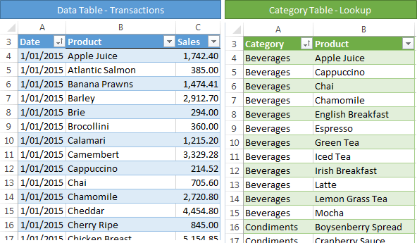
I’ve got two Excel tables [image 1], one for my transactional data (called ‘data’). If you’re familiar with databases, then this is often called a fact table. The other table is a list of my Products and their respective categories (called ‘categories’); this is the table you’d normally lookup to find the category for each product.

In the pre-Power Pivot days I’d use an INDEX & MATCH formula to bring the Category information into my Data table, but no more.

Power Pivot does VLOOKUP

Let’s look at how we can get our data into Power Pivot, create a relationship between the two tables and then analyse the data in a single PivotTable.

1. Make sure your data is formatted in an Excel table (CTRL+T). Mine are called ‘data’ and ‘categories’.
   Tip 1: It’s a good idea to rename your tables from the default of ‘Table1’, ‘Table2’ etc. as this name will also be used in Power Pivot.
   Tip 2: Your lookup table must not have any duplicate values for the Product column. Makes sense since Power Pivot wouldn’t know which record to choose if there was more than one.

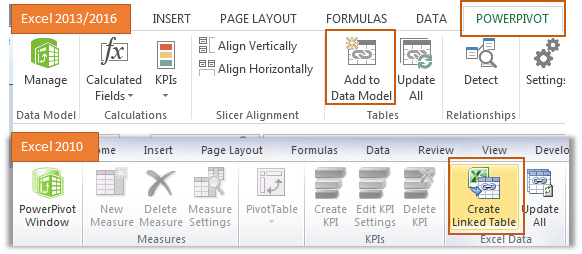
2. With any cell in your table selected, go to the Power Pivot tab > Add to Data Model (Excel 2013/2016) /Create Linked Table (Excel 2010) [image 2]:

This will open the Power Pivot window [image 3] and you can see your data table. It looks a lot like Excel with a formula bar, rows and columns and a ribbon with tabs etc.:

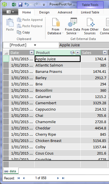
3. Repeat for all tables. Tip: Notice the name of the tables in Power Pivot is the same as the Excel Table names. In my example they are ‘data’ and ‘categories’.

4. Next we need to create the relationship between the two tables.
   
   

   If you’re familiar with VLOOKUP then you can think of it in the same way. For example, using VLOOKUP we’d add a column to the ‘data’ table that looks up the Product name from the data table, finds the matching name in the categories table and returns the category for that product (we’ll ignore the fact that we'd have to change the categories table column order to Product, then Category, for VLOOKUP to actually work, but you get the idea.

   In Power Pivot we simply tell it which table is doing the looking up, which the table is being looked up and which are the matching columns from both tables. Power Pivot doesn’t care what order your columns are in.

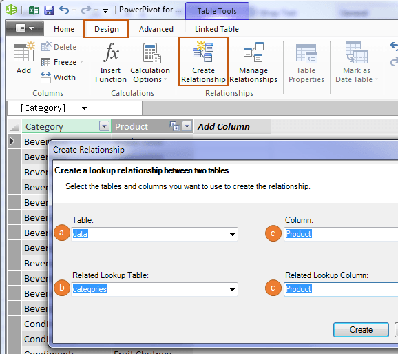
   To set up the relationship go to the Power Pivot window > Design tab > Create Relationship [image 4].

   (a) ‘Table’ is the one containing our transactional data, which is called ‘data’.

   (b) ‘Related Lookup Table’ is the table we’re looking up, just as you would with a VLOOKUP formula. In this example it’s the ‘categories’ table.

   (c) ‘Column’ and ‘Related Lookup Column’ are the matching (related) columns from each table. In this example, the Product columns. Remember: the Product column in the ‘Related Lookup Table’ cannot contain duplicate values in.

Grouping Dates in Power Pivot

One thing I’d like to be able to do is group my data by month. In Power Pivot for Excel 2010 and 2013 there is no Group functionality like we have in regular PivotTables. There is in Excel 2016 but I’m using Excel 2013, so, we can do this one of two ways;

1. Add a 'date' table to our model for date classifications, then create a relationship between the ‘data’ table and the ‘date’ table. This is the preferred method as it results in a smaller file because there is typically less data.
2. Add columns to our source data that classifies the dates into their month/year etc. I’m going to do that for this example to keep it simple, and because the Date table isn’t the focus of this tutorial.

Adding Columns in Power Pivot

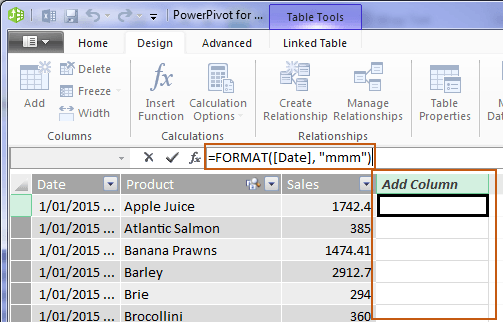
Adding a column for the month name is much like Excel.

In Power Pivot we have similar functions to Excel and they have similar syntax structure. For the Month name I’m going to use the FORMAT function to extract the month name from the Date column. In Excel we would use the TEXT function to do the same thing.

1. To add a column click in a cell in the ‘Add Column’ column of the ‘data’ table, or click on the ‘Add Column’ column header.
2. In the formula bar type your formula [see image 5].
3. Then press ENTER to complete it.

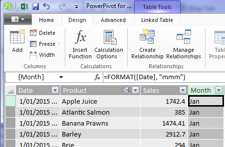
4. Double click the column header of your new column and give it a new name. I’ll call mine ‘Month’ [image 6].

Set ‘Sort by Column’ Rules

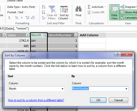
The month names we’ve just added are text, so when we use them in the Power Pivot PivotTable they will be sorted alphabetically instead of in month order. We can override this by telling Power Pivot to sort the month names based on the month number, but we need a column containing the month number first.

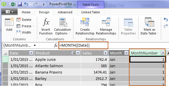
1. We’ll add another column and use the MONTH function (just like in Excel) to extract the month number from the Date column [image 7].

   

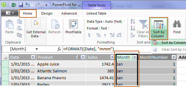
2. With the Month column selected go to the Home tab > Sort by Column [image 8]:

   

In the ‘Sort by Column’ dialog box [image 9] the Sort Column should already show ‘Month’ because you selected it before clicking ‘Sort by Column’. In the By Column choose ‘MonthNumber’:

Inserting a Power Pivot PivotTable

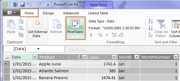
Now that we have our relationship set up and the extra columns for our month name and sorting rules we can insert a PivotTable. Power Pivot PivotTables are created from the Power Pivot window.

1. In the Power Pivot window > Home tab > PivotTable [image 10]:

2. In the Create PivotTable dialog box choose where you want to put the PivotTable; New or existing worksheet.
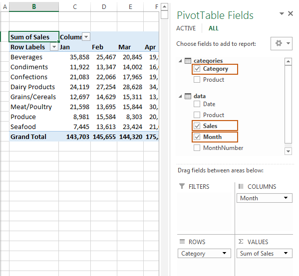
3. You should see both of your tables in the Field list. Clicking on the triangle (Excel 2013/2016) or + sign (Excel 2010) beside each table name will reveal the fields, and can go ahead and build your PivotTable using fields from both tables.

Step by Step Video

Wow, it seems like a lot of steps to replicate a VLOOKUP in Power Pivot but it’s actually not that involved. I’ve recorded a 2 minute video (no sound) so you can see how easy it is.

More on Power Pivot

• Get the free Power Pivot add-in
• Learn Power Pivot
• Learn Excel PivotTables - this is a must before learning Power Pivot.