Must-Know Excel Tools

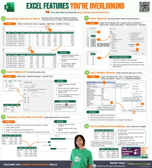
Hidden within Excel (sometimes in plain sight) are game-changing tools that most users overlook. In this post, I'm going to share 6 must-know Excel tools that will transform your productivity.

You can watch the video below or read on to learn more about these tools.

Must-know Excel Tools Video

Free Practice Workbook and Cheat Sheet

Must-Know Excel Tools You're Probably Not Using

1. Very Hidden Sheets

We often need to hide sheets in our workbooks to keep them tidy, prevent users from accidentally breaking formulas, or keep information confidential.

However, the common method of hiding sheets isn't very secure. Here's how you can make them more secure.

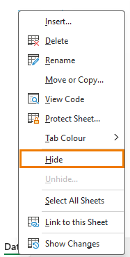
When you right-click a sheet tab and select Hide, it is no longer available to navigate to, which is great.

However, users can simply right-click again and choose 'unhide,' making the sheet visible.

To avoid this, you can protect the workbook structure, which prevents others from unhiding the sheets via the Review tab > Worksheet Protection, but that can be easily removed.

A more discreet method is using the Visual Basic Editor via the Developer tab.

Steps to Make Sheets Very Hidden:

1. Enable the Developer tab (if you don't already have it): Right-click the Ribbon > Customize Ribbon > Check 'Developer.'
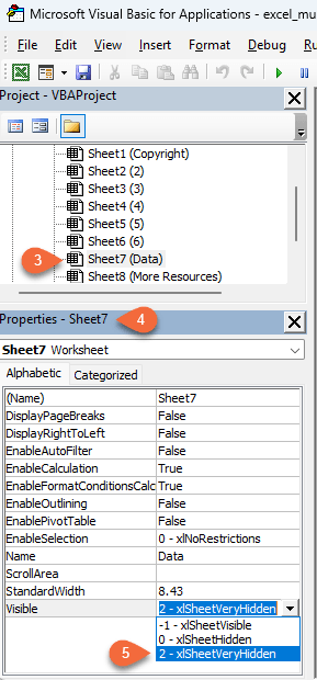
2. Open Visual Basic Editor: Developer tab > Visual Basic or press ALT+F11.
3. Select your sheet in the Visual Basic Editor.
4. Open the Properties pane: View > Properties.
5. Set the Visible property to 'XL sheet very hidden.'

Now, back in Excel, the sheet is hidden without any indication, reducing the temptation to snoop around your file.

Remember, Excel's protection isn't foolproof, so avoid using this for highly confidential data.

To unhide the sheet, go back to the Visual Basic editor (ALT+F11) and change the Visible setting for the sheet back to ‘-1 – xlSheetVisible’.

2. Paste Special (Convert Values)

Most people use Paste Special to paste formulas as values, but there are other super useful tools in the Paste Special dialog box that you might be missing out on.

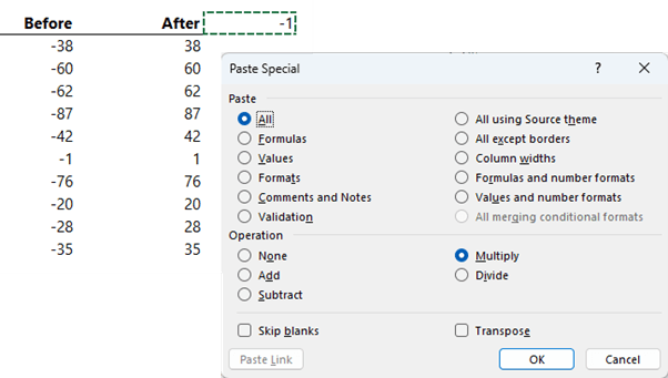
Example 1: Convert Negative Values to Positive

1. Enter -1 in an empty cell.
2. Copy it.
3. Select the range of negative values.
4. Use Home tab > Paste Special > Multiply.

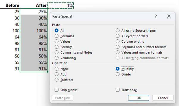
Example 2: Convert Values to Percentages

1. Enter 1% in an empty cell.
2. Copy it.
3. Select the range of values.
4. Use Home tab > Paste Special > Multiply.

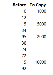
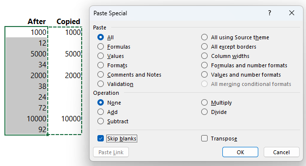
Example 3: Copy Values Without Blanks

1. Copy the range containing values and blanks.
2. Select the destination range.
3. Use Home tab > Paste Special > Skip Blanks.

Take some time to explore other Paste Special options for even more productivity boosts.

3. Clipboard

The copying and pasting tips don't end there. Normally, the clipboard clears when you perform another action. However, there's a way to store multiple items on the clipboard for pasting whenever you need.

Steps to Use Excel Clipboard:

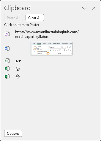
1. On the Home tab, click the Clipboard group launch icon:

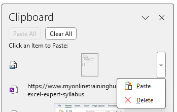
2. This opens the clipboard task pane, which stores up to the last 24 items you've copied or cut from any app:

You can delete items to keep the clipboard tidy:

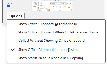
Or set options for how you want to work with the clipboard:

There's also a Windows clipboard you can open by pressing Windows button + V, which allows you to pin items for future use.

4. Group Data

When working with large spreadsheets, it can be helpful to hide rows or columns. If you find yourself repeatedly hiding and unhiding them, grouping is a better solution.

Steps to Group Data:

1. Select the rows or columns.
2. On the Data tab, click Group:

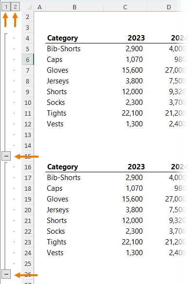
3. Use the minus button to collapse groups and the plus button to expand them:

You can add up to 8 levels of groups, allowing you to hide and unhide different sets of data.

To ungroup, select the grouped columns or rows and click Ungroup:

5. Custom Number Formats

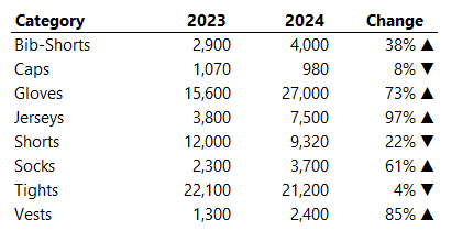
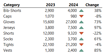
Interpreting key information in a sea of numbers can be time-consuming. Custom number formats can make your data more intuitive. For example, you can add symbols to indicate positive or negative changes.

Steps to Add Custom Number Formats:

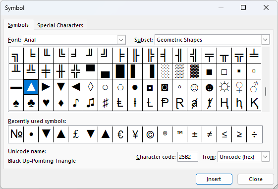
1. Insert the symbols into an empty cell from the Insert tab > Symbols. Make sure the font is Arial and the subset is Geometric Shapes:

Copy the symbols to the clipboard (CTRL+C)

2. Select the cells containing the data you want to format.
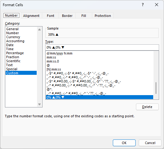
3. Press CTRL+1 to open the format cells dialog box.
4. Select Custom from the Category list.
5. Edit the Type field to include the symbols, e.g., 0% ▲;0% ▼.

Custom number formats are a vast topic with many possibilities. Download my comprehensive custom number format guide and cheat sheet.

6. Conditional Formatting

Conditional formatting helps quickly interpret data and identify patterns. For example, you can color code variances to make them more visually intuitive.

Steps to Apply Conditional Formatting:

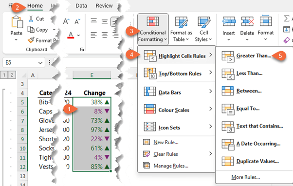
1. Select the cells you want to format.
2. On the Home tab, click Conditional Formatting.
3. Choose Highlight Cells Rules > Greater than and apply a custom format.

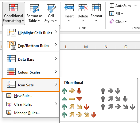
You can also use icons to visually indicate variances:

Just note that these icons aren't customizable in colour:

The upside of using symbols in custom number formats as opposed to conditional formatting, is symbols can also be used in chart labels, whereas conditional formatting cannot.

Conditional formatting has many built-in options, but the real power comes with using formulas to determine which cells have the formatting applied. Check out my other tutorial on using formulas for conditional formatting to learn more.

Master these hidden Excel tools to enhance your productivity and streamline your workflow.

If you'd like to learn more hidden gems like this to help streamline your work and stand out from the crowd, please consider my Excel Expert course.