Excel check boxes are a type of form control that can be added to a spreadsheet with just a few clicks to create an interactive list of items that can be checked off.
You can also link them to formulas to dynamically turn off and on items you want displayed in a chart or conditional formatting and more.
In this tutorial we’ll look at a few ways we can use check boxes to make your spreadsheets more visually appealing and user friendly.
Table of Contents
Watch the Excel Check Boxes Video

Download the Excel File
Enter your email address below to download the sample workbook.

Note: This is a .xlsx file please ensure your browser doesn't change the file extension on download.
Where to Find Excel Check Boxes
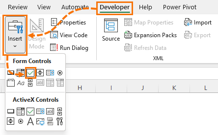
Excel check boxes are available from the Developer tab of the ribbon:
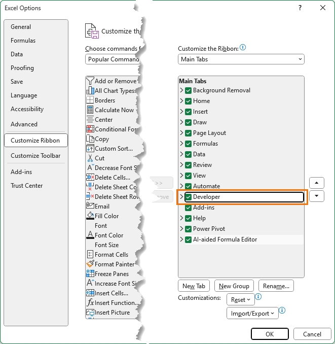
If you don’t see the Developer tab in your Ribbon, right-click the Ribbon > Customize and check the box for the Developer tab in the Main Tabs list:
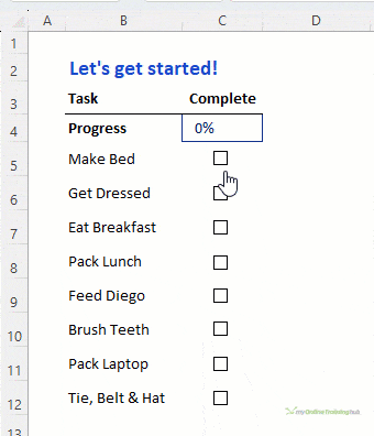
Excel Check Box Task List
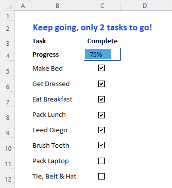
One of the most common uses for Excel check boxes is to create a task list you can use to keep track of progress.
I created one for my son’s morning routine before school because I’m tired of reminding him what he needs to do each morning, so I delegated it to Excel!
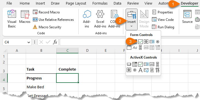
How to Build a Check Box Task List
Enter the list of tasks and then on the Developer tab > Insert > Check Box:
Draw the checkbox onto the cell beside the first task. Right click the text box > Edit Text:
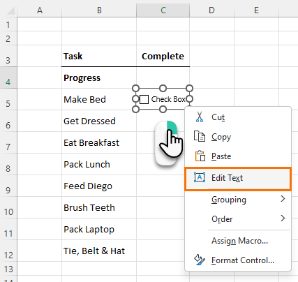
You could enter the task name here and do away with the need for the tasks in column B or simply delete the text box label, which is what I’ve done.
Next, resize the text box and place it in the centre of the cell. Then copy and paste the text box for the remaining tasks (watch the video above for tips on how to duplicate the text boxes and align them quickly).
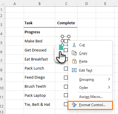
Next set up the cell link which returns the status of the check box.
Checked will return TRUE and unchecked will return FALSE.
Right click the text box > Format Control:
Select a cell to assign the text box status to in the Cell link field:
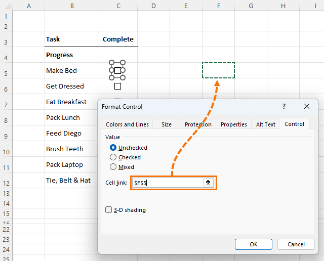
Tip: the cell link can be on any sheet in the file containing the check boxes.
Note: the cell will be blank until you check the box for the first time or select the ‘value’ in the Format Control dialog box shown above.
These TRUE and FALSE Boolean values can be used in formulas. When math operations are applied to a Boolean value, they are converted to their numeric equivalents of one and zero.
This means I can add a Progress Complete status bar using a formula to count the completed tasks divided by the count the total number of tasks:
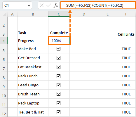
The formula above uses the double unary (- -) to coerce the Boolean values into their numeric equivalent.
See the video above for a more in-depth explanation and to see how I generate the custom message of encouragement in row 2:
Check Boxes Toggle Conditional Formatting On and Off
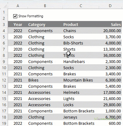
The check box is linked to cell F2.
The technique works because the Conditional Formatting formulas must return either TRUE or FALSE.
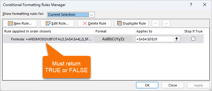
The formats are applied when the formatting rule formula returns TRUE.
We can therefore tie check boxes to conditional formatting rules to turn the formatting on and off by wrapping the Conditional Format formula in the AND function and referencing the check box cell link cell e.g.:
=AND(your conditional format rule, check box cell link cell)
If the check box linked cell contains FALSE, the format is not applied because the AND function only returns TRUE if both arguments are TRUE.
To shade every other row the Conditional Formatting formula is:
=AND(MOD(SUBTOTAL(3,$A$4:$A4),2),$F$2)
In English the formula reads:
- Count the number of visible rows in column A (that’s the SUBTOTAL(3… part, where 3 is the COUNTA function for SUBTOTAL)
- Divide the count SUBTOTAL returns by 2, and return the remainder, (that’s the MOD part), which will always evaluate to either 1 or zero
- AND check to see if cell F2 contains TRUE
I used the SUBTOTAL function because I only want to highlight visible rows and SUBTOTAL enables me to ignore hidden rows in the count. Learn more about the SUBTOTAL Function here.
The MOD function returns the remainder after a number is divided by a divisor. With 2 as the divisor of the count returned by SUBTOTAL, the result is either 1 or 0, which are the numeric equivalents for TRUE and FALSE required by the conditional formatting rule.
Finally, the AND function enables me to also see if the check box is checked. If the cell link contains FALSE, the conditional format is not applied.
Note: column A cannot have any blank cells, otherwise the count returned by SUBTOTAL will be wrong. In which case, choose a column that doesn’t have any blanks.
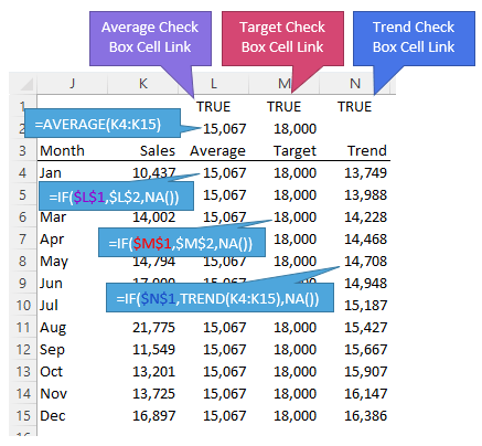
Check Boxes to Display/Hide Chart Series
Check boxes enable you to add interactive elements to charts, including and removing series at the click of a button.
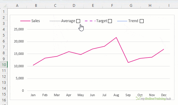
The source data from the chart is linked to the check box cell links. With all the check boxes checked, the table looks like this:
And with them unchecked, it looks like this:
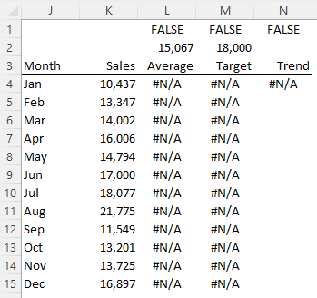
The Average, Target and Trend series are hidden in the chart because #N/A errors do not display in charts.
The IF function syntax is:
=IF(logical test, value if true, value if false)
The IF formulas simply reference the check box cell link in the first argument, with TRUE returning the value if true argument and FALSE returning the NA Function, which results in #N/A.
