Excel IF Formulas and What Not To Do

We can learn a lot from looking at what others do in Excel, both the good and the not so good. Last week one of my course members asked me to help them understand what a nested IF formula was doing in a file they’d inherited in their new job. It contained 15 nested IF functions, 5 CEILING functions and a load of repetition. The person who wrote this formula must have had one hell of a headache when they finished concocting it. Here it is:

=CEILING(IF(C11="consignment ",(IF($G11>30,(CEILING(IF($B11="Station A",IF($F11>10,($B$4-$D11+$F11),($B$4-$D11)),IF($F11>10,($B$5-$D11+$F11),($B$5-$D11))),10)+(H11-AGO/365*30*IntRate)),(CEILING(IF($B11="Station A",IF($F11>10,($B$4-$D11+$F11),($B$4-$D11)),IF($F11>10,($B$5-$D11+$F11),($B$5-$D11))),10)))+20),(IF($G11>30,(CEILING(IF($B11="Station A",IF($F11>10,($B$4-$D11+$F11),($B$4-$D11)),IF($F11>10,($B$5-$D11+$F11),($B$5-$D11))),10)+(H11-AGO/365*30*IntRate)),(CEILING(IF($B11="Station A",IF($F11>10,($B$4-$D11+$F11),($B$4-$D11)),IF($F11>10,($B$5-$D11+$F11),($B$5-$D11))),10))))),10)/FXRate

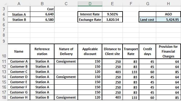
And here is the data on a sheet called 'Formula' (anonymised for confidentiality):

I re-wrote the formula and didn’t use any IFs! Not only is my formula way shorter, but it’s also much easier to decipher.

In this tutorial I’m going to:

• Step through the process I take to decipher complex formulas like this
• We’ll look at the avoidable mistakes they made writing the formula
• I’ll show you how to write a simpler formula that doesn’t contain any IFs!

Watch the Video

Download Workbook

Deciphering Formulas

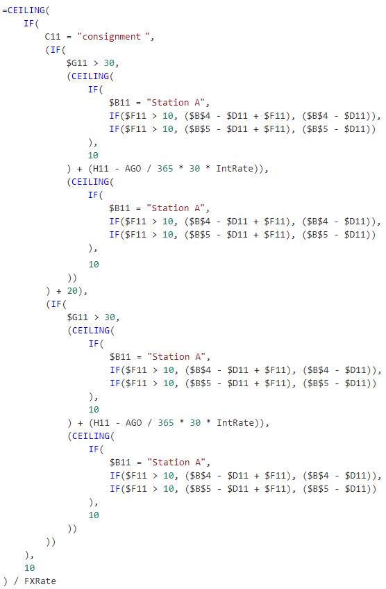
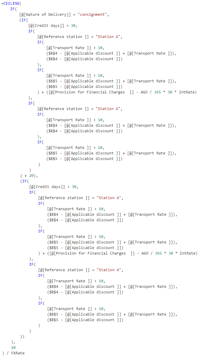
The first thing I did was copy the formula out of one of the cells and create it as a formula in the Advanced Formula Environment add-in (see video for more), which automatically adds line breaks and colour coding, making the formula easier to read:

Note: if you aren’t able to download the add-in, you can add your own line breaks inside the formula bar using ALT+ENTER.

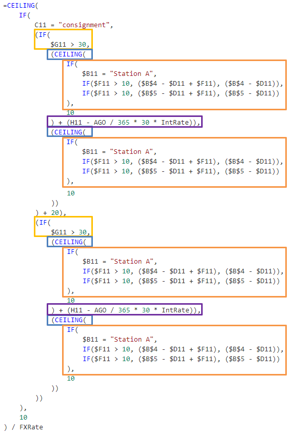
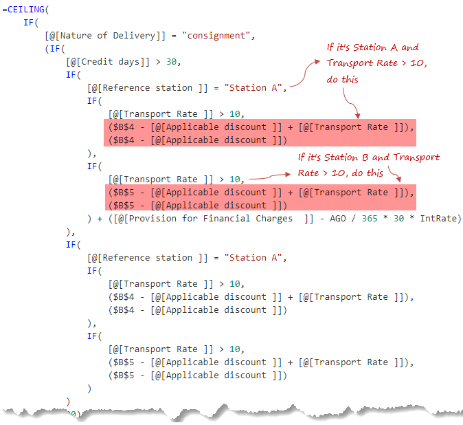
I could see the first IF formula criteria contained an extra space on the end of 'consignment ', which I corrected. You could also easily see there was a lot of repetition which I’ve enclosed in colour coded boxes below:

The CEILING function rounds numbers up to the nearest multiple of significance. In this formula it is rounding up to the nearest 10. Notice it is rounding twice, once at the IF level and again before converting with the foreign exchange rate. Given how this formula has been written and because this is a pricing model, as opposed to a scientific calculation, I put this down to user error as I doubt the intention is to round it up twice.

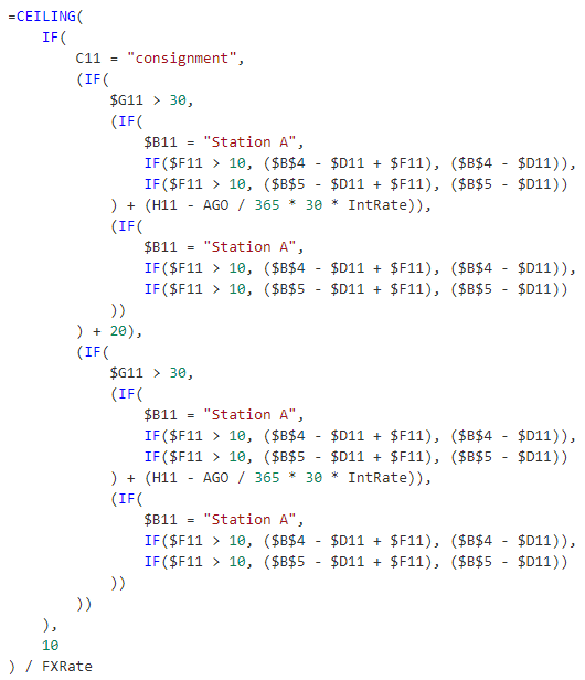
Below you can see that removing the internal CEILING functions reduces the noise a little. It results in a very small difference of 0.00262 or 0.15% for the first customer, which I expect is acceptable given the objective of this formula.

Format as Table

The next change I made was to convert the data to an Excel Table so that I could see the structured references rather than plain cell references, which instantly makes the formula readable in English:

Tip: To convert the cell references to the Table’s structured references, edit the formula and double click the cell references and then select the cell again in the table. Repeat for all references! Alternatively, you can use Find & Replace to replace the cell references in the formula with the Structured References, but I personally find it just as quick to replace them with the mouse.

Extract Criteria

Lastly, I isolated the various criteria so I could see the logic being applied. Here is the spreadsheet again so we can easily reference it:

There are 3 logical tests applicable to all scenarios:

1. If the Nature of Delivery in column C = consignment, add 20
2. If the Transport Rate in column F > 10, add the Transport Rate amount from column F
3. If the Credit Days in column G > 30, add the Provision for Financial Charges (col H), minus the Land Cost (in cell G5 named AGO)/365*30*Interest Rate in cell E4

These conditions apply to all customers therefore there’s no need to repeat them in multiple IFs. Instead, we can simply add them on at the end. More on that in a moment.

Repeating IFs

The last repeating IFs detect which Reference Station is in column B. If it’s Station A, the value in cell B4 is used, and if it’s Station B, the value in cell B5 is used. Otherwise, the formula is the same:

The author of this formula has used nested IFs to cycle through the different calculations for each station. A more efficient way is to use a lookup formula to find the value for the Reference Station and then add the other charges based on the logic identified earlier.

Lastly, the formula is wrapped in CEILING to round it up to a multiple of 10 and then divided by the Foreign Exchange Rate in cell E5, called FXRate:

Simplified Formula with NO IFs

Like I said earlier, an easier and more efficient way to write this formula is to use a lookup function to find the value for the station. Then we can add the other charges based on the criteria, apply the rounding with CEILING and convert the currency.

In the formula below you’ll notice that I haven’t used IF at all:

=CEILING(
   XLOOKUP([@[Reference station ]],$A$4:$A$5,$B$4:$B$5,,0)
   -[@[Applicable discount ]]
   +([@[Nature of Delivery]]="Consignment")*20
   +([@[Transport Rate ]]>10)*[@[Transport Rate ]]
   +([@[Credit days]]>30)* ([@[Provision for Financial Charges ]]- AGO/365*30*IntRate)
,10)
/FXRate

Note: if you don’t have XLOOKUP, you can use VLOOKUP or INDEX & MATCH instead.

The arguments in blue are Boolean logical tests, if the test is TRUE, it returns the numeric equivalent of 1, which is then multiplied by the respective values/calculations. If the test returns FALSE, it returns 0 and 0 multiplied by anything is 0.

Taking the first logical test as an example: ([@[Nature of Delivery]]="Consignment")*20

In English it reads: if the nature of delivery is ‘Consignment’, the logical test returns 1, multiplied by 20 = 20

I could have written these as IFs, but it’s not necessary. For example, the above line could be written:

IF(([@[Nature of Delivery]]="Consignment", 20, 0)

In English the whole formula reads:

1) Lookup the reference station in cells A4:A5 and return the cost in column B.

2) Take off the value in the Applicable Discount column.

3) Plus, if the Nature of Delivery is consignment, add 20.

4) Plus, if the Transport Rate is greater than 10, add the Transport Rate amount.

5) Plus, if the Credit Days are greater than 30, take the value in the Provision for Financial Charges column, minus the AGO amount, divided by 365, times by 30, times by the Interest Rate.

6) Round up the value so far to the nearest 10

7) And finally, divide the final amount by the Foreign Exchange Rate.

Lessons Learned

1. While some functions can perform the same calculations that others can, it doesn’t mean they’re the best ones to use. It’s important to know a range of functions so you can choose the correct function for the task. Check out my Advanced Formulas course here.

2. Structure your formula with carriage returns so they’re easier to read.

3. Format your data in an Excel Table so you can use the structured references, which makes formulas readable in English.

4. You don’t always need IF to apply a logical test.