G'day Team,
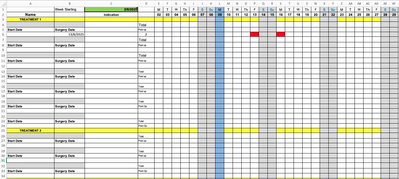
My first post here so be gentle. I have been an Excel user since 1993 and was a train the trainer back in the ADF for many years, so a little bit of background in it. But saying that, so much under the hood that I learn something new every week. But this problem has me stumped. The workbook is used to track patients in my unit by the nurses but it could be for anything. I have attached a screen shot of the workbook for visual reference.
I am attempting to use conditional formatting to shade in cells that a person is unavailable. The top rows are the days of the month, formatted to show the day number only, feed from the date entered in C1. In column B is a date the person is not available. I also have the number of days the person is away in Col D. So what I am looking at is when nurse enters surgery date, CF looks at cell in B and Row 2 to see if true and if it is add the number of days (NETWORKDAYS) to B cell date and shade in those dates on that row. I have a project planner that shades between two dates but I need to use the KISS principle as the nurses have issues working out the auto fill function in excel.
Thanking everyone in advance.
Not sure if I've understood as the screen shot doesn't match the text in your question. B2 is empty, though B6 seems to have a date that triggers some CF. The attached file might help you on your way. If not, please come back and upload your file and manually colour the cels to show how CF should do it.
Not sure if I've understood as the screen shot doesn't match the text in your question. B2 is empty, though B6 seems to have a date that triggers some CF. The attached file might help you on your way. If not, please come back and upload your file and manually colour the cels to show how CF should do it.
Riny,
Sorry for the confusion, I was referencing the B column as a whole and the Row 2 as a whole but can see how that might be taken as B2.
That said I may have worked out a workaround using a WORKDAY formula to a hidden cell and using that to shade in. Doing some clean up testing and will report back. Thanks for the sheet, I will review and see if cleaner than my work around.
Riny,
Perfect and much cleaner than the work around I did. Looking at the formula I was almost there but nowhere close enough. A big thanks.
Ok, I have had a play around and attached is the result. A big thanks to Riny for the solution.
Attached is the file with the Riny CF using =E$2=MEDIAN(E$2,$B1,WORKDAY($B1,$D1)-1) I never would have thought of using MEDIAN.
I also included my work around in tab TROY CF with =AND(E$2>=$B4,E$2<=$AH4) AH4 is where I have a formula =WORKDAY(B6,D6) This cell would be hidden so not accidentally deleted. For some reason the cells shade in two cells up, not on the line of the date. Not sure why but that is the line the nurses normal write on when printed so not too concerned.
I also have CF to shade in holidays which I coloured in a different shade to weekends. On the example the 9th of June is Kings Birthday holiday here in Australia. I have this hidden normally as well. I think it is about as simplistic as I can get it given the target users.

