Hello,
I have a Pivot Table with an associated Chart, and a slicer. I don't want all the fields from the table so I can filter some out, but the slicer still shows all the fields. Can I get the slicer to reflect the number of fields from the filtered table?
In the image, he Adopter Profile field is filtered and the chart is correct. How can I change the slicer to reflect the changes on the filter
![]()
Thanks and HAPPY NEW YEAR to everybody. Hopefully with these new vaccines coming along we can get back to some normality sooner rather than later.
[Image Can Not Be Found]
Hi Robert,
In Excel 2016 and later you can set the Slicer settings to 'hide items with no data' so that when you have other filters applied which result in items in the Slicer not being present in the PivotTable/Chart they won't appear in the Slicer list. You can access the settings by right-clicking the Slicer > Settings.
Mynda
Thank you Mynda. I will try that.
Happy New Year to you and your wonderful team.
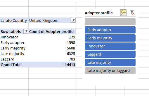
Hi Mynda, I'm coming back about this filter problem with slicers.
I have been reviewing your recent video about the dashboard for non-financial data - wonderful, thank you.
I have a pivot table and sorted the Row labels manually, and filtered, and so hidden two of the rows. Both these rows are non-zero values so the option to 'hide items with no data' does not work here. I would like the Slicer to now reflect the sorted and filtered pivot table. You can see the 'offending' slices are coloured grey. I would like these slices to be hidden, and the list of slices to be in the same order as in the pivot table. Is all this possible, please? I am using Excel 365.

Thank you.
Hi Robert,
The only way to hide the items from the Slicers is to remove them from your source data. As for sorting the Slicer items based on the PivotTable, you can either create a custom list, or use the technique I demonstrated in the Dashboard video where I use the Sort By setting in Power Pivot.
Mynda
Ah. OK. Thank you very much for getting back so soon.
