Slicers are a fantastic tool to get a filtered view of your data and visuals.
But by default, they get sorted alphabetically or follow the calendar year if your parameter contains months.
What if you wanted them sorted in a custom order? Maybe you want to show fiscal years, a Sunday to Monday work week or just any specific order your whimsical boss tells you to?
No need to panic, you can sort slicers any which way you want, just follow these nifty tricks!
Table of Contents
- Custom Sort Slicers Video & Workbook
- Exploring the Sample Data
- Default Slicer Sorting Dilemma
- Sorting Fiscal Months (with Custom Lists)
- Sort Single Slicer for Month and Year (using helper Columns)
- Sort Date Slicers - Data Model (Date Table)
- Sort By Column – Data Model (Custom Sorting Text Labels)
- Choosing the Best Method
- What's Next
Watch the Video

Download Workbook
Enter your email address below to download the example files.

Exploring the Sample Data
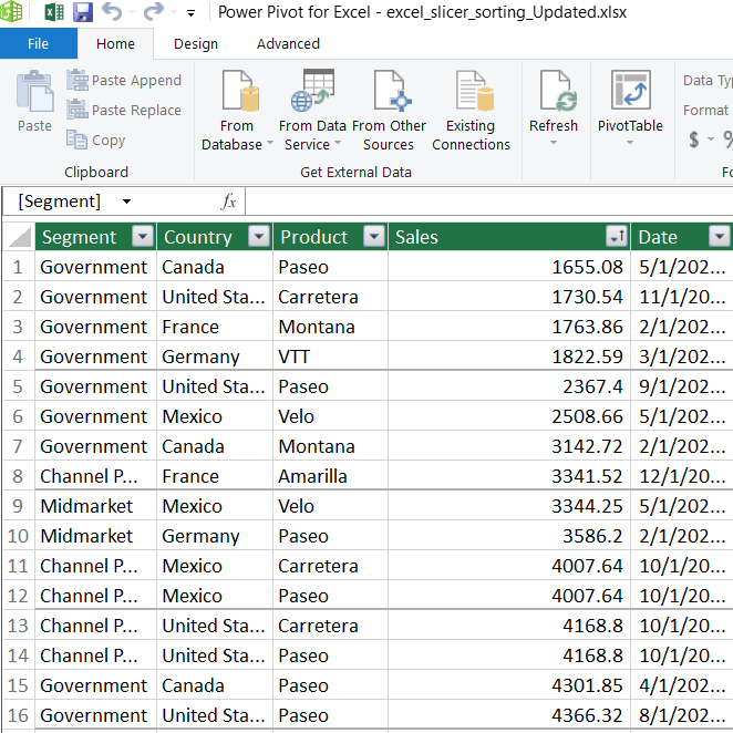
Here we have a sample dataset that shows the Sales, of 6 products on any particular date between July 2022 and June 2023, segregated by Segments and Country.
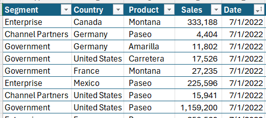
With this data, we can easily calculate the monthly, quarterly, and yearly sales during the financial year, or answer questions like “What are the total sales from France?” or “How much Sales does the Government Segment bring?” And so on.
To do such an analysis, we will use pivot tables, slicers, and pivot charts.
The Default Slicer Sorting Dilemma
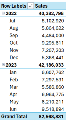
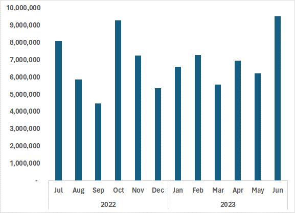
Suppose we want to look at monthly sales during the financial year starting from July 1, 2022, to June 30, 2023.
Let’s follow the below steps:
- Insert a pivot table with years and months in rows and sales in columns
- Insert a pivot chart to visualize the data
- Insert a slicer for this pivot table
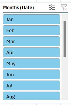
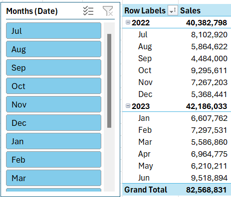
While the pivot table and the chart sort correctly from July to June, by default, the slicer sorts from January to December.
Why does this happen?
The reason why slicers sort from January to December is that we can only add one field at a time in a slicer. While the pivot table incorporates both years and months to get the right sorting order, the slicer can only pick months because our data set includes grouped dates in mm-dd-yyyy format.
Why is this a problem?
Default sorting could be misleading, making the viewer believe that there weren’t any sales from July to January.
Fiscal Month Custom Sorting
Fiscal year is the standard accounting and taxation period used to calculate various decision-making performance metrics, such as profitability and MoM, QoQ, or YoY changes, for any business. Therefore, most businesses prefer having their data and visuals, including slicers, sorted according to the fiscal year.
However, in most countries fiscal year and calendar year have different start and end dates. For example, Australia follows a July to June fiscal year, The US follows an October to September fiscal year and India follows an April to March fiscal year.
Therefore, our slicers need to be sorted accordingly. We can achieve this using several methods, the simplest of which is the Custom Lists method.
Custom Lists method
To add a custom list, follow the below steps:
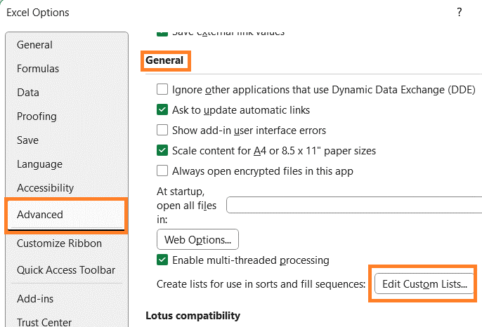
- Click on the File tab
- Go to Options
- Select Advanced tab
- Scroll to the General heading towards the bottom
- Click on the Edit Custom Lists button
Here you can add your own custom sorting order.
There are two methods of doing it:
- Manually type your sorting order, by comma separating each value
- Importing your list from a cell range in your Excel file
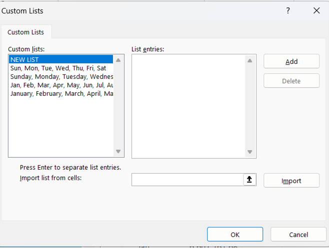
Once you have added the custom list, press ok and refresh your Pivot Tables. The slicer should sort in the required custom order.
While the fiscal year is just one application of custom-sorted slicers, the same procedure can be used for varying work weeks. For example, a week starting from Sunday to Monday, instead of the standard Monday to Sunday format.
Limitations of the Custom Lists method
Although this is a simple method, it has several limitations:
- The list doesn't automatically grow as you add more data: While months are known beforehand you might need to use a different sorting parameter, such as the country of sale. Every time you have a new country added to the dataset, you will have to add it to the custom list.
- Limited items are allowed: You can only add up to 2,000 items to your custom list
- Non-Transferable: Every time you transfer the file to a new computer, you will have to add the custom list to that computer for the correct sorting order.
- Format limitations: Custom lists can only contain text or alphanumeric data. If you want a custom list containing only numbers you will need to first create the list of numbers and then format it as text.
Sort Single Slicer for Month-Year
As we pointed out above, slicers can only have one field at a time. And with all the limitations of the Custom Lists method, it is not always the best option.
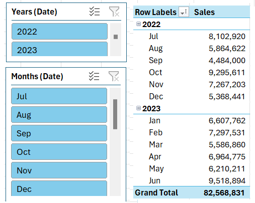
If you want to avoid the Custom Lists method, and you still want to have grouped dates in your dataset, you will need to have two slicers in place – one for the year and one for the month.
Even so, you will have to look at individual years if your fiscal year is split across two years. Which is not only cumbersome, it doesn’t give the insights for the entire year.
But hold on! There can be a sneaky workaround for incorporating both year and month in the same slicer!
Here are the steps to follow:
- Create a helper column to your dataset, call it Period
- Copy the grouped dates to this column
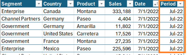
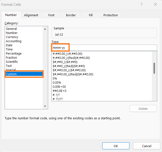
- Select the Period column and Press CTRL+1 to open the Format Cells dialog box
- Choose Custom from the Category list
- Enter the mmm-yy format in the ‘Type’ field
This will format the period column dates to show months and years in a single column. You can use this new column in the slicers!
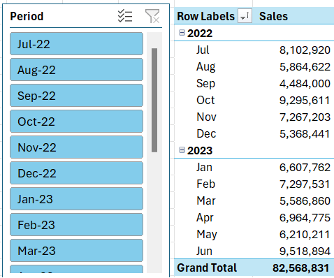
Now, why is this method sneaky, you ask? It's because your pivot table and chart don't get affected. They still use the date column but your slicers are sorted in the Fiscal Year sorting order!

If you want your data to show months and days instead of months and years, you can format it as mmm-dd to get the desired results too.
Limitations of Sneaky Workaround
While this is a much simpler method compared to Custom Lists, it too has its limitations. When you work with larger data sets, the helper column causes your file to become very heavy. This could lead to longer file opening time or longer load time for visuals.
To avoid such issues, you can use the more advanced Data Model Method to sort your slicers, as explained below. Using this method, you can sort in almost any order you want. We will cover 2 such examples – Fiscal Year Sorting & Segment Sorting.
Sort Date Slicers - Data Model (Date Table)
As explained before, most businesses want the sorting to be in Fiscal Year order. You can achieve it by using the data model method. Here are the steps:
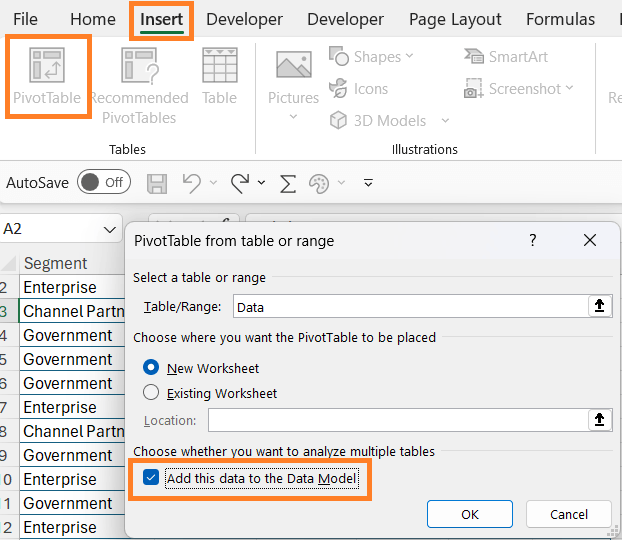
- Go to Insert tab
- Insert Pivot Table but before pressing ok on the dialog box, checkmark the "Add this to the Data Model" option
- Press ok
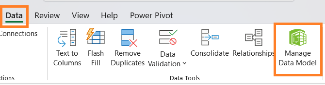
- Now go to the Data tab
- Select the Manage Data Option
A new window will open showing the data view of your data.
From here, follow the below steps:
- Go to the Design tab
- Click on Date Table
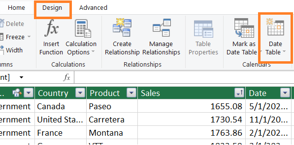
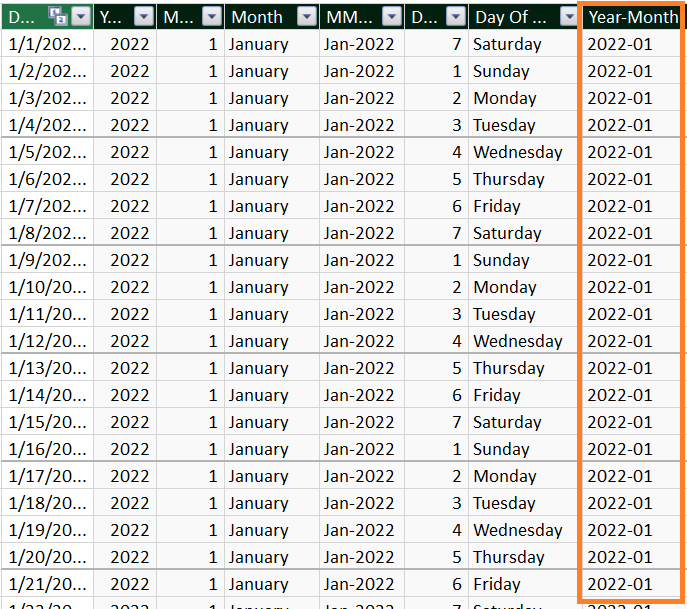
This will create a new table called the "Calendar" table. It automatically analyses the smallest and the largest dates in your data set and creates a relevant table. This table automatically contains the MMM-YYYY column.
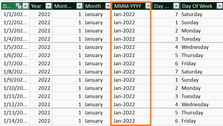
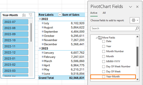
However, if you use this in your Pivot Tables, it will sort alphabetically. Therefore, you need to add a column that concatenates the year and month fields in a YYYY-MM format. This way it will automatically sort in the correct order. To do that, click on the first cell of the add column and in the formula bar type the below formula.
='Calendar'[Year]&"-"&FORMAT('Calendar'[Month Number],"00")
This will give you the desired format for your slicers. You can also rename this column as Year-Month.
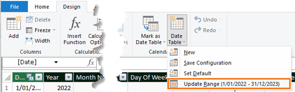
Tip: If you ever need to add dates to the calendar table, you can do so via the Design tab > Date Table > Update Range:
Next, you need to connect this calendar table to your data table. For that follow the below steps:
- Got to the Home tab in the Data Model
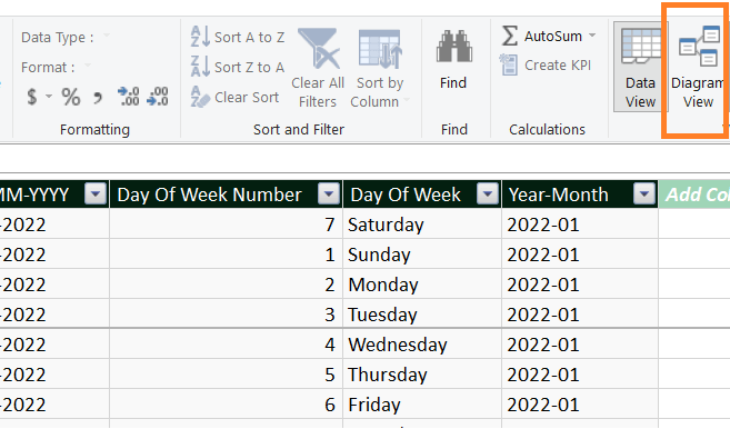
- Click on Diagram View to see both data and calendar tables
- Drag the date from the Calendar table to the data table to create a connection between the two tables. Note: Don’t make the reverse connection. The Calendar table should filter the Data table, not the other way round. The relationship should have the arrow on the connector line pointing towards the data table.
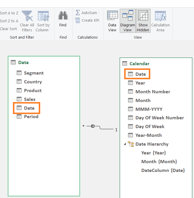
- Also, to avoid using the date field from the data table in your PivotTables, right-click on it and click on "Hide from Client tools."
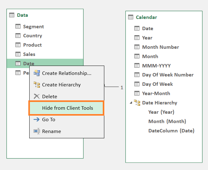
- Save the Data Model and close it.
Now create your pivot table taking the Date Hierarchy from the Calendar table, and Sales from the Data Table.
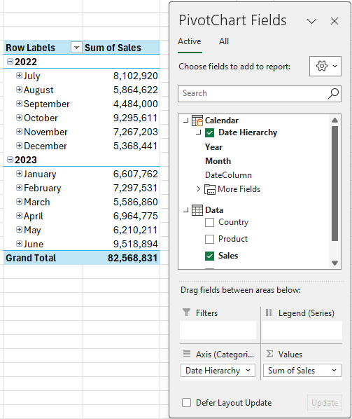
Insert a Slicer using the Year-Month field and it will be sorted in the Fiscal Year order because the data starts in July 2022.
Advantages of the Data Model Method:
While it takes time to get used to this method it has several advantages:
- It works best with large datasets.
- You don't need to recreate it on every computer you open the file.
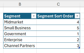
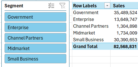
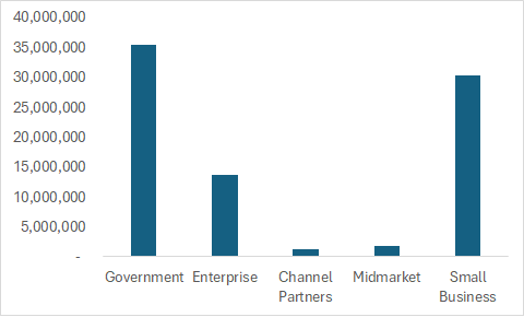
Segment Sorting: Data Model
Suppose your boss wants you to sort the sales Segment-wise, not fiscal year-wise and you don't want to use the Custom Lists method because you have too many segments to work with. You can use the Data model Method for this also.
For example, let’s say we want the Segment order to be: Government, Enterprise, Channel Partners, Midmarket, and Small Business respectively.
Here are the steps to sort the slicers in the desired order:
- Create a new table in the Excel file with 2 columns Segment & Segment Sort Order
- Populate the table with unique Segments and the sort order you want.
Next, we need to add this Segment table to the data model. We can follow the same steps as explained in the previous example.
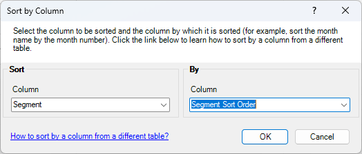
Once the segment table is in the Data model, we need to set the sort order:
- Select the Segment column and on the Home tab, click on the Sort by button:
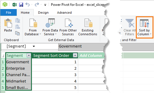
- In the dialog box, Sort Column should be Segment and Sort By column should be Segment Sort Order.
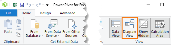
- Go to the Diagram view:
- Drag Segment field from the Segment table and drop it on the Segment field in the Data table, to create the connection. (Don’t make the reverse connection. Segment table should filter the Data table)
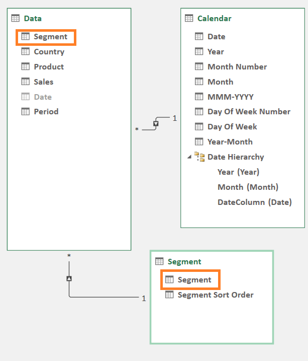
- Hide Segment in the Data table from client tools.
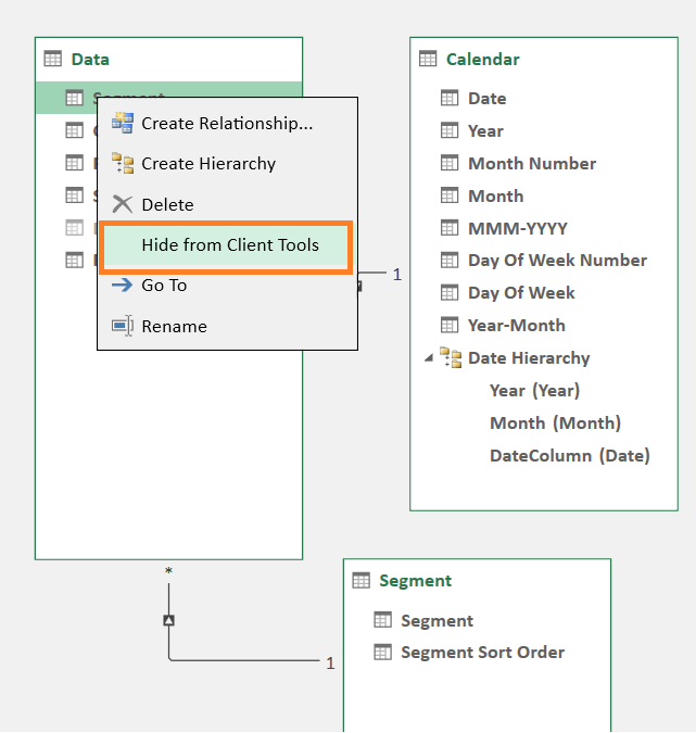
- Save the Data Model and close it.
- Add Segment to rows in your pivot table from the Segment table and Sales from the Data table.
- Insert a slicer for Segments and it will be sorted in your desired order!
Limitations of the Data Model Method:
While it makes sorting much easier, it has its own limitations:
- It is a little complicated to set up.
- Table connections need to be correct to make it work.
- At times you might need to use DAX formulas which are not so straightforward.
Which is Best?
Overall, all three methods are very useful when custom sorting slicers, but you need to decide which is the best method for you. Guidelines:
- Use the Custom Lists method when you have a small dataset, your sort-by list doesn't expand, and you don't need to view the file to different computers.
- Use the Sneaky Workaround method when you have a small dataset and you just want a single date slicer for year and month. This method travels with the file, so there’s no extra set up for different computers.
- Use the Data Model method when you have a large dataset, your sort-by list doesn’t expand, and you need to transfer the file to different computers.
You can use the Data Model method even if your sort-by list expands, by using Power Query to create an automatically updating sort-by list.
Let me know in the comments which method you think is best and why.
What's Next
More Power Pivot: This has been a glimpse into the additional capabilities Power Pivot offers over regular PivotTables, including far more flexibility and capacity to work with large datasets spread across multiple tables.
The bonus of learning Power Pivot is it’s available in both Excel and Power BI, so the skills are transferrable. You can learn more about Power Pivot formulas in my Power Pivot and DAX course.

Slicer Formatting Hacks: Now that you’ve got your Slicers sorting the way you want, it’s time to learn some formatting hacks in the video below to make them small so they don’t take up so much space.


hello,
thanks for your description.
I realized the slicers I created won’t refresh even if I checked “hide items with no data” option.
In fact “(blank)” field is still in, even if I replaced all the blank cells with data.
I read somewhere to stop Excel from showing deleted items in a Slicer, I should select the Slicer and then click Slicer Tools > Options > Slicer > Slicer Settings. I should then be able to uncheck Show items deleted from the data source and click OK.
My problem is I cannot find that option in my Slicers settings !! I find only 3 options: 1 hide items with no data; 2 Visually indicate items with no data; 3 Show items with no data last.
Another strange thing is that if I go to PivotTable Options >Data ,
1 “Save source data with file” option is unchecked and greyed out;
2 “Retain items deleted from the data source” is set on Automatic and the field is greyed out.
I tried to create new worksheet, new pivot tables and slicers and everything is the same.
I use Office365 proPlus.
Any suggestions? I spent a lot of hours without finding any solution 🙁
Hi Mark,
It sounds like you may have added your data to the data model/Power Pivot? Please post your question and Excel file on our forum where we can help you further.
Mynda
Right!
I created multipled pivots table from multiple tables. That’s why I selected the field “add this data to the data model”.
I made a test.
I just created new table with few rows and columns. Then I created new pivot table without selecting “add this data to the data model”. In this way I verified I was able to select “none” in “Retain items deleted from the data source section”.
Then I created a slicer. Even in this case I was able to check “show items deleted from the data source”.
In my case, how can I refresh all the slicers?
thanks
Hi Mark,
Please post your question and file on our forum. It’s not clear what you mean by ‘refresh all the slicers’? They should all be in sync if they are all connected to the same PivotTables.
Mynda
Hi Mark,
Can we see your file? If possible, please remove sensitive information from the file and upload it on our forum (create a new topic after sign-up).
It might be a Power Pivot, not just a regular pivot table.
Hello,
How can You create the bar on the top (overview, Team view, sport view)?
Hi Mark,
These are just shapes with hyperlinks.
Mynda
Hi,
When forwarding a excel document to other people then the custom list will not appear anymore.
Is there a solution to that?
Thank you
Hi JP,
No, unfortunately you need to create the custom list on each PC. That’s why I tend to use the other option.
Mynda
Plan B didn’t work for me. My slicer insists on using the dd-mmm format even though the source column has mmm-yy format and still gets the order wrong. Yes I refreshed the pivot table. Thankfully the pivot table and pivot chart have the dates in the correct order despite the stupidity of the slicer. What you didn’t make clear was how the data in column “Period” was entered. Did you use the same data from the first column just changed the format or did you enter the data in the third column as mmm-dd. By the way, my slicer also has tons of other dates (not highlighted) which are not connected to any data when I click on them.
Hi Dave,
Did you insert a new Slicer using the new mmm-yy column?
I explain how I created the extra column in the post above starting with this sentence: “To get around this we simply add another column to our Source data which contains the same dates from column A, except this time we format them with a Custom Number format mmm-dd….”
Also, if you download the Excel file you can see how I added the column.
Greyed out buttons in your Slicer represent data that is not present in the PivotTable at the current filter level. You can turn this off in the Slicer settings (right-click the Slicer).
If you have no filters applied, but still have greyed out buttons then they represent data you used to have in your PivotTable source data that is no longer be there. To remove that data, right-click the PivotTable > Options > Data tab > set ‘Number of items to retain per field’ to ‘None’.
Let me know if you still have problems.
Mynda
i don’t have the option of “use custom list when sorting”.
why is that ? what to do ?
Hi Yahel,
If you check the box ‘Load to Data Model’ when creating your PivotTable then your data is actually stored in Power Pivot and your PivotTables are Power Pivot PivotTables. Slicers for Power Pivot do not have the ability to sort using a custom list.
For Power Pivot you need to add a numeric column to the dimension table containing your Slicer items and use the ‘Sort by’ tool in Power Pivot to sort the Slicer items column by your numeric column. If you get stuck, please post your question and sample Excel file on our Forum where we can help you further.
Mynda
This is a great article, Mynda! Do you know if there is any way to work with slicers and alphanumeric labels? I am building a dashboard of several different numbered promotions and need both the number and promotion name. The slicer obviously tries to sort as if the numbers are text (i.e. 1, 10, 2, etc.), which makes using them difficult. Any idea of a workaround? I’m not finding anything on the internet otherwise. I’m also using Excel 2010 btw.
Hi Alex,
Have you tried to build a custom list with the correct order of your values?
Mixed type values will indeed be sorted alphabetically, in this case you better put promotion name before the numbers, it will sort better.
Thanks, Catalin! I considered a custom list but know those have to be created on each computer viewing the file, and I don’t understand VBA well enough to auto-apply them. Unfortunately, I will be emailing this file to multiple parties, so it seems like this would not be practical. I appreciate your suggestions, though!
It’s a simple code:
Sub AddCustomList()

 Dim n As Byte, ArrList As Variant

ArrList = Array("983711", "TM 2516", "980261", "TM5660", "78011", "983712", "TM2517", "980263", "TM5661", "78012", "EF810028", "6060", "XSR", "985221", "TM2452", "15AL1630", "HD21A", "H25")

On Error Resume Next

n = Application.GetCustomListNum(ArrList)

On Error GoTo 0

If n = 0 Then

    Application.AddCustomList ArrList

    n = Application.CustomListCount

End If

End Sub
Finally I have my slicers in order!
Love the sneaky workaround.
Thanks
Wonderful! Glad you found it useful 🙂
Mynda, Is the Custom Sort Slicer Setting not applicable to Powerpivot Pivot Tables?
In Power Pivot we have other ways to sort Slicers, namely ‘Sort by’.
Hello
very nice post, thank you for sharing.
I’m using Excel 2013 and slicers. The data source is in percent but the slicer is showing the numeric values. So even though it says 29,1% in the column in the pivot table, the slicer shows 0,291. Some slicer values have up to a dozen decimals and it does not look very good. It seems formating the slicer is not possible, using the ctrl + 1 command. Any workaround?
Hi Patrick,
You’ll need to add a column to your source data that converts the percentages to text. You’ll then use that column for your Slicer, but the actual percent column in your PivotTable.
If you get stuck please post your question on our Excel Forum and include a sample Excel workbook so we can show you.
Mynda
Hi Mynda
that worked fine, thanks for helping!
Have a nice day.
Hi, I was wondering if you could help, when I group my days in the pivot table, it shifts the dates by 1 days. i.e. if I have 1st Jan,1st Jan, 2nd Jan, 2nd Jan, 2nd Jan, 3rd Jan and then I go to group it – it changes the dates in pivot table to 2nd Jan, 3rd Jan – 1st jan disappears. Any ideas?
Thank you
Hi Jay,
I’ve not heard of that before. Can you please post your question on our Excel forum where you can upload a sample file so we can take a look.
Thanks,
Mynda
A nice solution IF the person designing the pivot table will be the only one using it, and only using it on one computer. The fact that the custom list needs to be set up on any computer using the table makes this unusable for my purposes. I typically distribute these kinds of tables to a number of faculty members.Would love to see Microsoft address this with an intuitive, drag-and-drop solution.
Hi John,
I guess the ‘nice solution’ you are referring to is the Custom Lists. I agree, these aren’t ideal, that’s why I recommend Plan B in my post above.
Mynda
Hi,
Need enter manual value in slicer.
Help on it.
Hi Ajit,
The only way to get an item appear in your Slicer is to have it in your PivotTable source data. You could always create a dummy PivotTable for the purpose of your Slicer.
Mynda
I have created Pivot table and I want to use slicer in my baseboard.
But in that slice more than 800000 entry. It is very difficult to find single value.
Please help me.
thanks
Ajit K.
8483842013.
Sounds like you’re using Slicers for the wrong type of data. If you have 800,000 unique items then you probably should be grouping them somehow so you can make sense of the data.
HOW TO MAKE SCLICER FOR DAY WISE FOR eg-
day 1
day2
day-3
for every day i have different price so i want to make upto 50 days, day wise price sclicer.
kindly help me in this
Hi,
You have to add a new column to the data table, and use a simple formula like this: =DAY(Table1[Date])
Refresh the pivot table, and you will be able to add this field to a slicer.
Cheers,
Catalin
I report sales to various Cities. Alphabetical sorts are fine, but my Pivot Chart is sorted by volume sold to the city and I’d like the slicer to be sorted in the same order, ie The city with the highest volume, which is the first bar on the chart, should be on top. As different slicer date rages are selected, the sort order changes. I don’t see a way to use the sneaky workaround because of this. Do you?
Hi Tim,
Nope, there’s no way to dynamically sort Slicers. The best you can do is use a custom list to sort the Slicer the way you want but that won’t update upon changes in the items selected.
Kind regards,
Mynda
Hi Mynda, When I open up my slicer settings I do not have the “Use Custom Lists when sorting” option. I’m working in Excel 2013. Is there an add-on to have that option? Right now I only have “Data source order” above the ascending and descending options. I appreciate your assistance with this. Thank you, Angie
Hi Angie,
That’s odd. There’s no add-on but you might have an old version of Excel 2013? You could try upgrading to the latest build for 2013.
Mynda
Hello,
Indeed, actually I have the same issue with Excel 2016. I don’t have the “Use Custom Lists when sorting” tick box you mention. Only Sort A to Z, Z to A and “Data source order” which I haven’t figured out yet… I’ll keep digging but if anyone has any ideas?
Thanks!
Laure-Emmanuelle
Hi Laure-Emmanuelle,
I have the check box to ‘use custom lists when sorting’ in my version of Excel 2016. Are you using a Mac?
Mynda
I have the same problem and I am using Windows 10, Excel 2016. The checkbox for custom lists is not there. Just the option buttons. Interestingly enough, when I open Mynda’s file the option box is there, but not on my own
Hi Bill,
That’s odd. If you right-click the PivotTable > Options > Totals & Filters tab, do you have a ‘Use Custom Lists when sorting’ checkbox available under the ‘Sorting’ heading?
Mynda
Great article, and I can’t wait to try this with some of my own data!
I’m a great fan of the Olympics, and I’m intrigued by the dashboard you show. Is there a place to get a copy of it? I would love to be able to access it as I watch the 2016 Rio Olympics!
Hi Wanda,
Thanks for your kind words. I’m delighted you like my dashboard. You can get a copy of it in my Excel Dashboard Course:
https://www.myonlinetraininghub.com/excel-dashboard-course
Alternatively you can ask Shane Devenshire for a copy of the raw data.
Kind regards,
Mynda
Thanks! I found it!
I think the real problem is that your dates are not actually dates; they are text. Apply the formula DATEVALUE() to your dates to convert them to a number which can be formatted as a short or long date. Then the dates will sort properly since they are in numerical order.
Hi Will,
The dates are real dates but the minute you group those dates in the PivotTable using the Group tool the PivotTable considers them text (and you cannot avoid this), so you must use one of the workarounds described above.
Mynda
I know this is an older article, I used the workaround feature which works fine if you have only 1 entry for that specific date , if you have multiple dates and then try to group them it goes back to the original format, is there a workaround for this when you multiple entries for the same date ? Thanks in advance.
Hi Eric,
The solution is to add a column to your source data with the grouping in a text format and then use this field in your PivotTable report. Here is a tutorial that explains it in more detail:
https://www.myonlinetraininghub.com/create-a-single-excel-slicer-for-year-and-month
Kind regards,
Mynda
You are a gem ! Works like magic
Thanks, Vilas 🙂
Thanks for this. What about sorting dates without slicers? I have data from July 2013 to July 2014 in the columns. And I want Excel to sort the columns in Financial Year order, July to June then July to June again?
Hi Cathy,
I’d probably be inclined to use the Custom List for two reasons:
1. since it’s something you would need to use on a regular basis the effort required to install it on all computers that would use it wouldn’t go to waste.
2. With the ‘Sneaky Workaround’ option you’d have to create a column of numeric values. e.g.
July would be 201401
August would be 201402
September would be 201403
And so on, just so you could sort the months in the order you want. This column could be hidden in your PivotTable report but since it’s not intuitive it may lead to confusion.
Kind regards,
Mynda
Great post. It worked perfectly. Thanks for sharing.
You’re welcome, Jef 🙂
Hi Mynda,
Thanks for the tips.
I believe maybe there is a typo… should be “mmm-yy” be “mmm-dd”?
“To get around this we simply add another column to our Source data which contains the same dates from column A, except this time we format them with a Custom Number format mmm-yy.”
Well spotted MF. Thanks for letting me know. It’s all fixed now.
Cheers
Mynda
Another note:
When I added the newly formatted date field, and added that slicer to the pivotchart, in order to get the pivotchart to update, I had to delete the Period slicer, otherwise it would not add the new data to the chart, even though it would add the dates to the slicer.
Hi Glenn,
I suspect the two Slicers were in conflict, so that would make sense that you have to delete one of them.
Cheers,
Mynda
Mynda:
I found this to be an interesting article. However, for me, one big drawback is the fact that the custom list has to be updated if you add data.
So here’s a suggestion: Rather than add the Period sneaky workaround, why not just define a custom date format of yyyy-mm-dd and use that in the data table and for the slicer? This will sort properly, and it will update if you add more data to the table and refresh the Pivottables. The only downside is that there may be some confusion as to the date format, especially with international audiences, but if the custom Date header is something like “Date: YYYY-MM-DD” that would address that concern. (As a note, I find the format in your “Period” slicer to be confusing; I initially read that as month-year rather than as month-day, so the issue already exists to some extent…)
Thanks for the stimulating discussion.
—Glenn
Hi Glenn,
I agree with the drawback for the custom list which I why I proposed the Sneaky Workaround.
If you use Date column (A) in your PivotTable/Chart and group those dates, and then use that same field for your Slicer, you end up with the dates not sorted correctly.
This is why I suggested the ‘Sneaky Workaround’; that is to add an extra column of dates (C), which are formatted as you wish (mmm-dd or yyyy-mm-dd etc.), and then you use this column for your Slicer. I believe this is the same as your proposal?
I agree you could change the heading of column C to make the date format clearer, or you can simply give the Slicer a different name in the settings.
Kind regards,
Mynda
Just a page report: I noticed that the last section saying “Share This” is not activated when I am clicking it. For example if I click Pinterest it does not pop-up.
Maybe I am the one who is not using it well. That was just a notice. You can delete this comment when you are done reading it.
Good job Mynda and Phil.
Hi Maxime,
Not sure what is happening for you. When I try the Pinterest in the ‘Share This’ section, it works for me. I tried all the social sharing buttons and they all work for me.
Have you got a pop-up blocker turned on? Each of the social sharing buttons tries to open a pop-up window.
Regards
Phil
It is not working Phil. I do not know what was wrong with it yesterday. Maybe something on my end.
Thank you for your reply.
hmmm. odd. what browser are you using? Can you try another browser? Chrome, Firefox or Internet Explorer.
I just have the Excel 2013 installed and Slicers was the first thing that I know I would learn. This article is very helpful. Many thanks to MyOnlineTrainingHub.com.
Mynda or Phil, I would like another article showing how to have the Slicers listed horizontally instead of vertically.
Many thanks!
Hi Maxime,
Glad you liked Slicers too. I realised as I was writing this that I hadn’t written about them before so I will plan some more tutorials 🙂
In the meantime you can make Slicers horizontal by changing the number of columns in them. Go to the Slicer Tools: Options tab of the ribbon, which is available when the Slicer is selected, and in the Buttons group you can increase the number of columns. Then drag the pull handles of the Slicer to make it horizontal.
Kind regards,
Mynda
Horizontal slicers worked!
Thank you for the tutorial. Have a wonderful day.
You’re welcome, Maxime 🙂 You have a wonderful day too!