Format your dashboards and reports fast with these pro Excel chart formatting tips.
Watch the Video

Pro Tip 1 – Select Multiple: Hold the SHIFT or CTRL key to select/de-select multiple charts or objects.
Pro Tip 2 – Select All: Select one chart then press CTRL+A to select all. Note: This will select all Objects so if you have shapes or images in your worksheet it will select them as well.
With all charts selected you can move, resize, align, group, delete, copy, right-click and set properties including size, locking and more:
Pro Tip 3 – Snap to Grid: Hold down the ALT key while resizing and moving to snap to the grid:
Bonus tip: You can move and resize multiple charts at the same time.
Pro Tip 4 – Distribute Evenly: Select 3 or more charts > Format tab > Align > Distribute Vertically or Horizontally:
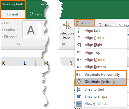
While you’re there you can also align them all left or right, or top/bottom.
Bonus tip: This is great for aligning any object, e.g. form controls, shapes etc.
Pro Tip 5 – Lock Alignment while Moving: Hold the SHIFT key while you left-click and drag to keep your chart aligned to its original horizontal or vertical position (useful it you’re not using the grid for alignment):
Pro Tip 6 – Repeat Formatting: Let’s say you decide that you want to remove the chart border from all your charts.
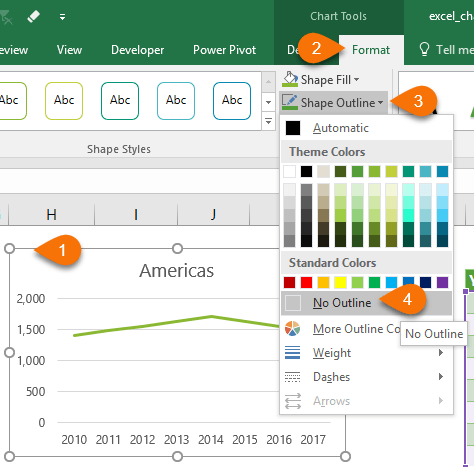
Make the formatting change to one chart, then select the next chart and press F4. Rinse and Repeat for remaining charts. This works for other formatting too.
Pro Tip 7 – Themes: Change all formatting in one go with Excel Themes. Choose from the built-in themes:
Or customize your own including colors, font styles and shape effects. Click here to learn how to use Excel Themes.
Pro Tip 8 – Duplicate/Copy Charts: Copy an existing chart with keyboard shortcut CTRL+D or left-click to select the outer edge of the chart > hold the CTRL key until the mouse pointer displays a + symbol, then left click and drag while holding CTRL.
Bonus tip: hold SHIFT at the same time to keep the new chart aligned to the one you’re copying:
Pro Tip 9 – Chart Templates: Got a chart you’ve spent considerable time formatting to just the way you like it and now use it all the time. Make it a chart template so it’s on call when you need.
Pro Tip 10 – Move Chart with Arrow Keys: Hold CTRL while left clicking the outer edge of your chart. Note: in Excel 2016 you no longer need to press CTRL, just a left click will do. The pull handles will be small dots which indicates that you can move the chart with your arrow keys:
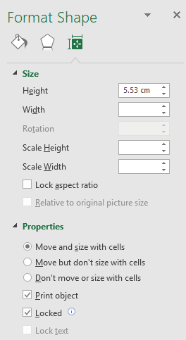
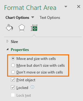
Pro Tip 11 – Prevent Charts Resizing: By default, charts will resize and move when you adjust column width and row height, but you can prevent this in the Properties. Right-click the chart > Format Chart Area > Properties:
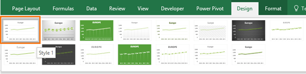
Pro Tip 12 – Don’t Use Built in Chart Styles: All but the default, Style 1, is generally a bad idea. They’re full of noise like unnecessary formatting and fill:
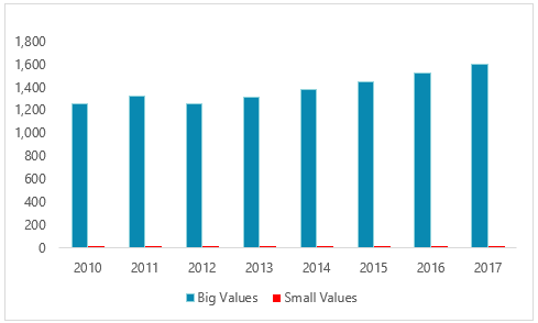
Pro Tip 13 – Select Chart Elements: Sometimes selecting the element you want can be tricky, like the ‘Small Values’ series in the chart below:
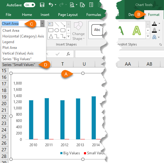
There are two options for selecting those teeny tiny chart elements:
- Select an element that’s easy to click on, like the ‘Big Values’ column > hold the CTRL key and press the up/down arrows to toggle through the other elements in the chart until you get to the one you want. Note: pre Excel 2016 you don't need to hold the CTRL key.
- Select the chart > Chart Tools: Format tab > choose the element from the drop down:
Pro Tip 14 – Copy All Formatting: If you want to copy the formatting from one chart to others, you can simply select the chart you want to copy formatting from > CTRL+C, then select the chart you want to copy formatting to > go to the Home tab > Paste > Paste Special > Formats:
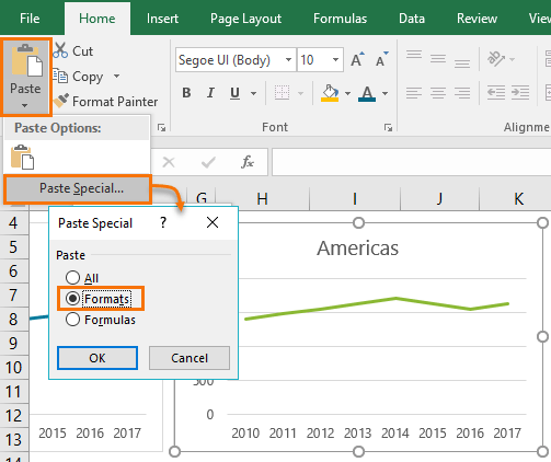
Note: Paste Special doesn't work with Pivot Charts. Instead, you can simply copy and paste, which will paste the formatting.
Please Share
If you liked this please click the buttons below to share.


Hi Mynda
I have developed a “Combo” chart with stacked Columns and Stacked Area and have linked the underlying pivot tables to slicers. Now on changing the slicer selection these charts reformat themselves and all series are displayed as Stacked area.
How can we stop this? I have tried changing the Advances Options not to change “Properties follow chart data point for current workbook” as well as for all new workbooks – as some websites propose.
PS I have also tried creating a Chart template, as you propose further down in this chat, but this does not help. One needs to change the chart type each time the format goes awry.
Hi Keith,
You can try applying the chart settings with no filters/items selected in the Slicers, i.e. in a completely unfiltered state. If that doesn’t work then this is the result of a known bug with Pivot charts. The solution is to insert a regular chart based on the PivotTable data.
Mynda
Hi, Mynda Treacy; Nice job on these tips! I copied some website info (a mix of text, pictures and graphics) into Excel-2016. I have everything the way I want it, but cannot delete the graphics. When they are clicked-on, they don’t have/display resizing dots at their edges and when I right-click on them, the context (or, right-click) menu doesn’t display at all. The graphics are small rectangular boxes that had embedded links in them in the website; in effect, they were “Click Here to Do This or That” buttons.
Do you have any suggestions to delete these annoying objects? They make what is otherwise a well-organized spreadsheet, quite messy looking. I can’t be the only one with this problem. Thanks for any assistance.
Hi Richard,
Maybe these objects are actually inside the cells. Have you tried deleting the cells or the contents of the cells? A better way is to use Power Query to get data from the web. If you’re still stuck, please post your question on our Excel forum where you can also upload a sample file and we can help you further.
Mynda
Tip 14 does not work? I cannot paste special after I copy a chart.
Hi Anna, It looks like something is preventing the paste special working with Pivot Charts in the latest version of Excel as it works with earlier versions of Excel and also works with regular charts, as you can see from the screenshot. I’ll raise a bug with Microsoft. In the meantime you can simply copy the chart and paste, which will paste the formatting. Mynda
Does not answer the question of keeping format (series names, colors, date range, etc,) from one graph to next
Series names and date ranges are not formats. These are dictated by the data your chart is based on.
Thank you so much for the valuable stuff.
You’re welcome
hi Mynda, With the help of your dashboard course I have been able to make myself a very usable Dashboard c/w 3 main chart areas and 3 slicers controlling them. It displays my sales dollars per year, per territory etc. The issue I am having is after I format the line colors to match in the 3 charts e.g. 2016 = red, 2017 = blue, 2018 = green, the line colors randomly change and when I refresh the data, I’ll end up with Chart 1 & 2 as Red, Blue Green but Chart # 3 may end up with Red, Blue Purple…… My numbers come up accurately based on slicer selections …so everything appears connected…. I’m not sure how to phrase the question – why do my line colors seem to have a mind of their own? Thx Tom D. Ontario Canada
Hi Tom,
This is a common issue with Pivot Charts resetting formatting upon filtering/Slicing. You could try creating a custom color theme for the chart and applying that, otherwise the colors are likely to reset each time a series is filtered out and back in again.
Mynda
Hello Mynda, hello Tom,
almost three years since the original post.
I have a similar problem with keeping line colors.
Is MS refusing to accept this as a mistake/error?
It is really frustrating that lines loose their color when refreshed / changed by slicer choice.
Or is there, three years after, now a solution?
Y’all have a great day
Steve
Hi Steve,
The problem is caused when the PivotTable is filtered to a point where the series is no longer present in the PivotTable. The Chart can’t remember the formatting for a series that is no longer there. So, if your filters completely filter out a series the best option is to create a regular chart from a PivotTable where you can ensure the cells referenced by the chart for each series are never removed. Instead they simply contain errors or empty cells.
Mynda
Hi Mynda, I’m trying to format a pivot chart title to include filtered text from the slicer along with the descriptor (and include a source in tiny font as a separate line below)… is there a way to do this? It only seems to allow me to either insert text – in which case I can format it as wanted – or insert linked cells – in which case it will only allow me to apply one default text to the whole??
here’s my eg as it might be a bit hard to follow: oops – this comment box only allows a default text also… [Actual] from slicer cost change over time 2011 – 2017 $m
(source, FIM)
if you can shed any light, would be greatly appreciated! thanks, Fran
L.E.:
oops, I seem to have worked it out – dah!
oh dear, no I haven’t – that was the unlinked text!
Hi Fran,
When you use a linked cell for chart title, you can only format the entire text, not just parts of it, as you already noticed. This happens in formulas too, different formats cannot be applied to formula results.
You can try a different method:
prepare your data in 2 or 3 different cells, format each cell as you want, copy those cells and paste them as linked picture from paste special menu, you can place this image on your chart replacing the title, it will update whenever you use the slicer. Calculation should be set to automatic.
thanks, that is helpful, however I do not know how to set calculation to automatic. I’ve searched all of the properties on the linked picture and simply cannot work it out. Help please…
It’s not a property of Linked Picture, it’s the workbook calculation settings. Look in the Formulas tab in ribbon, Calculation group->Calculation Options. It should be Automatic by default. If this is set to Manual, the linked picture will not update.
my calculation option is set to automatic, however the linked picture is not updating??
L.E.:
oops, sorry to bother you, have just realised that I must have stuffed it up somehow, as I redid it and it now works…
thanks very much for the assistance.
You’re welcome, glad to hear you managed to make it work!
No shorthand tricks but, in keeping with Mynda’s minimalistic style, I find that charts often appear better without any fill or border to the chart area. This allows the plot area to be better integrated with surrounding objects. That, of course, assumes that cell boundaries are not displayed in the vicinity of charts, shapes and controls.
As a personal style note, I would add that all sheets are improved by removing both the grid and the headings but that is more a style of working than a recommendation..
Great points, Peter. Maybe I should write a design tips post next.
Tip 2 and 5 is extremely useful as many are not aware of this trick.
As for tip 13.1, I don’t think it is necessary to press CTRL+arrow key (or am I missing something as I am using Excel 2010).
Just pressing the up/down/left/right arrow key (after selecting the element) should do it.
The up/down key select the series while left/right key will select each point/series.
Hi Sunny,
In Excel 2016 you now have to press CTRL with the arrow keys and since this also works in earlier versions I left it as is, rather than explaining the differences.
Mynda
You put the ‘Joy’ in the holiday season!
🙂 thanks, Allan!
this is very great and helpful. thank you
Thanks! Glad you like it, Abayomi 🙂