
Most Excel users are not aware that curly braces can be used inside functions like DATE, XLOOKUP, and SORT to name a few, to unlock behaviour that is otherwise hidden. These are not tricks or edge cases. They are built into how Excel evaluates formulas.
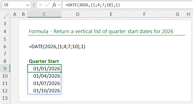
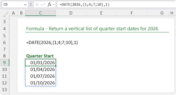
Just take the DATE function which most think returns a single date; you can see below I’ve used it to return the quarter start dates for 2026, and I’ll cover how and why it works in more detail shortly:
In this article, you will learn how curly braces work, why they matter, and how to use them in practical formulas you can apply immediately.
Table of Contents
- Watch the Excel Curly Braces Video
- Download Workbook
- What Are Curly Braces in Excel?
- Using Curly Braces With the DATE Function
- Filtering Specific Columns Using FILTER and CHOOSE
- Creating a Mini Summary Table With VSTACK
- Using Curly Braces in XLOOKUP for Smarter Fallback Results
- Multi-Level Sorting With SORT and Curly Braces
- Cleaning Messy Text With TEXTSPLIT and Multiple Delimiters
- Taking This Further With Advanced Excel Formulas
Watch the Step-by-step Video

Download the Practice File
Enter your email address below to download the free file.

What Are Curly Braces in Excel?
Curly braces define what Excel calls an array constant. You can think of an array constant as a small list of values that lives directly inside a formula.
For example:
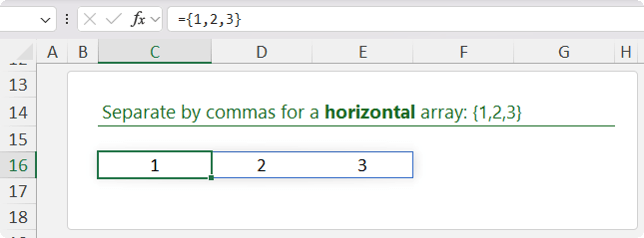
{1,2,3}
This is a horizontal array of three values:
Many Excel functions can accept arrays as arguments, even though most users only ever pass a single value. Once you understand this, you start to see Excel functions very differently.
In Excel 365, formulas that return arrays will usually spill automatically into neighbouring cells. The curly braces are simply defining the input values.
There is one important rule to remember when working with array constants.
Semicolons separate rows.
Commas separate columns.
This means:
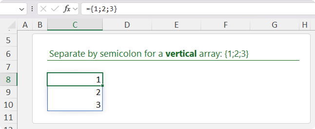
{1;2;3}
creates a vertical list:
While:
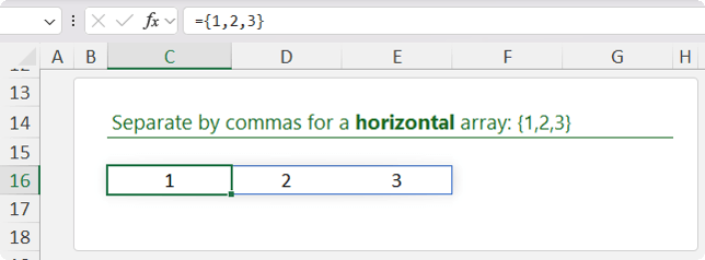
{1,2,3}
creates a horizontal list:
With that foundation in place, let’s look at how curly braces work inside real Excel functions.
Using Curly Braces With the DATE Function
The DATE function normally takes a single year, month and day
=DATE(year, month, day)
Most users expect it to return a single date.
However, if you pass an array of months using curly braces, DATE will return multiple dates.
For example, to generate quarter start dates for 2026:
=DATE(2026,{1;4;7;10},1)
Because semicolons are used, the results spill vertically. This instantly produces a list of quarterly start dates:
If you want the same dates to spill horizontally instead, use commas:
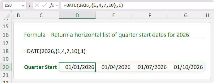
=DATE(2026,{1,4,7,10},1)
By changing nothing but the separators, you control the shape of the output:
This technique is perfect for building reporting periods or schedules without typing month lists onto the worksheet.
Filtering Specific Columns Using FILTER and CHOOSE
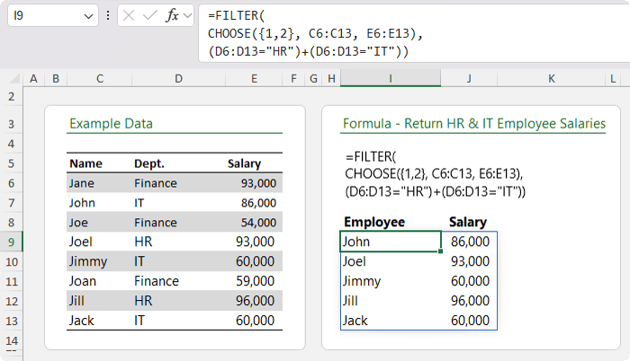
Suppose you have a table containing employee names, departments and salaries, and you want to return only HR and IT employees. That part is easy with the FILTER function .
But what if you also want to control which columns are returned, or even rearrange them, without creating helper columns?
This is where the CHOOSE function and curly braces come in.
Here is the full formula:
=FILTER(
 CHOOSE({1,2}, C6:C13, E6:E13),
 (D6:D13="HR")+(D6:D13="IT")
)
And here’s the result:
Let’s break this down.
The CHOOSE function is used to build a virtual table. By passing {1,2} as the index argument, you are telling Excel that you want two columns returned.
Next, you specify which columns those are. In this case, column C contains names and column E contains salaries. The department column in D is skipped entirely.
Finally, FILTER is used to return only rows where the department is HR or IT. The plus sign acts as OR logic.
This pattern is extremely powerful. You can use CHOOSE not only to select columns, but also to reorder them before they are filtered.
Creating a Mini Summary Table With VSTACK
Curly braces are also useful for building small summary tables without PivotTables or helper ranges.
For example, we can use VSTACK with COUNTIF to count how many employees are in IT and HR and display the result as a table:
=VSTACK(
 {"IT","HR"},
 COUNTIF(D6:D13,{"IT","HR"})
)
And here is the result:
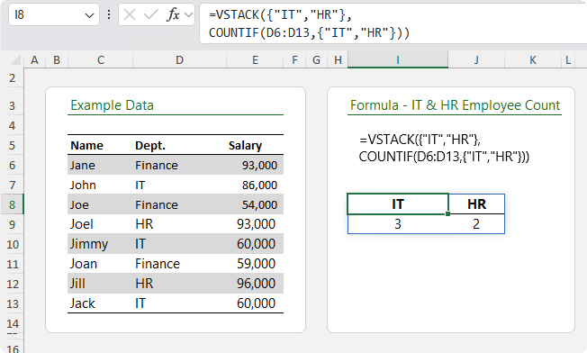
The first array constant: {"IT","HR"}, defines the labels. The COUNTIF function then accepts the same array constant as its criteria and returns both counts in one calculation.
VSTACK combines the labels and counts into a clean two-row table.
This is a simple but very practical reporting technique.
Using Curly Braces in XLOOKUP for Smarter Fallback Results
Most users know that the XLOOKUP function can return multiple columns. What many people do not realise is that the if_not_found argument can also return multiple values when you use curly braces.
Here is an example:
=XLOOKUP(
 I8,
 C6:C13,
 D6:E13,
 {"Unknown Dept.","Unknown Salary"}
)
This formula looks up an employee name in cell I8. If the name is found, it returns the department and salary.
If the name is not found, instead of returning a generic error or message, it returns a tailored fallback message for each column.
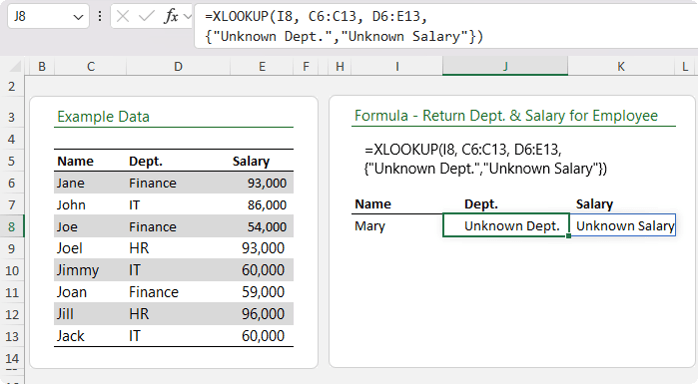
This results in much cleaner, more professional output, especially in reports or dashboards.
Multi-Level Sorting With SORT and Curly Braces
The SORT function can perform multi-level sorting if you pass a list of sort keys using curly braces.
For example:
=SORT(C9:G17,{2,5},-1)
Here’s the result:
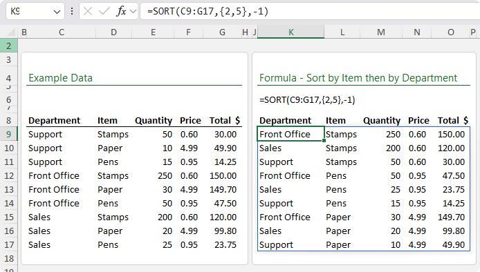
Here, {2,5} tells Excel to sort first by the second column and then by the fifth column. The -1 specifies descending order.
This allows you to perform complex sorts without SORTBY or helper columns, simply by passing an array of sort keys.
Cleaning Messy Text With TEXTSPLIT and Multiple Delimiters
The TEXTSPLIT function becomes far more powerful when combined with curly braces.
If you have a text string that contains multiple delimiters such as commas, slashes and parentheses, you can split it in one go.
For example:
=TEXTSPLIT(D5,{",","/","("},")",TRUE)
Here it is applied to a practical example:
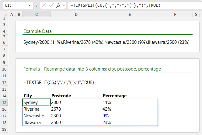
In this formula:
- The array constant: {",","/","("} defines multiple column delimiters.
- The closing parenthesis is used as a row delimiter.
- TRUE tells Excel to ignore empty values.
With a single formula, a messy block of text is transformed into structured columns.
Taking This Further With Advanced Excel Formulas
If you’re reading this and thinking, “I know Excel formulas, but clearly not like this,” that is exactly why I created my Advanced Excel Formulas course.
The course further into array logic, lookup patterns and modern formula techniques like the ones shown here, all grounded in real-world use cases.
You can find the course here: Advanced Excel Formulas Course


NitPicky of me, I know, but in your TEXTSPLIT example the Postcode and Percent are separated by a space and a parenthesis. and your formula only acts on the parenthesis, so the Postcode winds up with a space after it. Adding that space to your formula corrects for that.
=TEXTSPLIT(D5,{“,”,”/”,” (“},”)”,TRUE)
Good catch, Jomili!
You can also return multiple results with VLOOKUP with the assistance of curly braces, e.g.
=VLOOKUP(A1,B1:E10,{2,4})
This is an instance in which VLOOKUP’s solution is more elegant than XLOOKUP’s:
=XLOOKUP(A1,B1:B10,CHOOSECOLS(B1:E10,2,4))
Yes, good point. Thanks for sharing, Abbott! Be sure to add FALSE in the last argument for that VLOOKUP unless your data is sorted and you’re happy with an approximate match.