In today's fast-paced world, staying organized is more crucial than ever. With countless tasks to juggle, it often feels like we're spinning plates just to keep up.
But what if there was a way to make your life a little easier with an Excel calendar that updates itself, highlights your busiest weeks, and flags upcoming deadlines? Sounds too good to be true? Well, it's not!
In this guide, I'll walk you through creating a dynamic Excel calendar that you can use year after year.

Table of Contents
Watch the Step-by-step Video

Get the Dynamic Excel Calendar File
Enter your email address below to download the sample workbook.

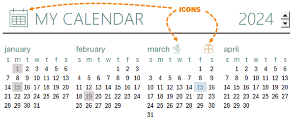
Why a Dynamic Excel Calendar?
A dynamic calendar in Excel is more than just a tool to keep track of dates. With features like conditional formatting, it can automatically highlight important events, such as holidays, birthdays, and deadlines.
Plus, it's incredibly easy to update for the new year with just a click of a button. This flexibility makes it an indispensable tool for anyone looking to stay organized.
Creating the Layout
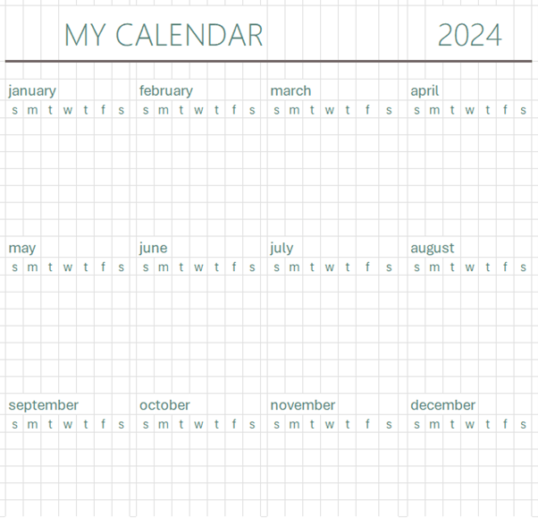
To begin, we'll create a new Excel file. My calendar is a 4 x 3 grid, but you can have any configuration you like.
1. Select Your Columns:
Start by selecting the columns (A:AF) where your dates will be displayed.
Adjust the column width to 2.7 to ensure everything fits neatly.
2. Set Up Your Year and Heading:
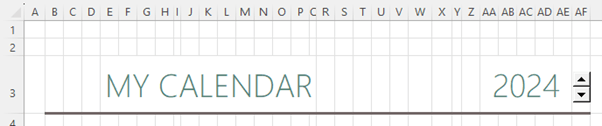
In cell AA3, enter the current year. Select cells AA3:AE3 and format the alignment to 'center across selection':
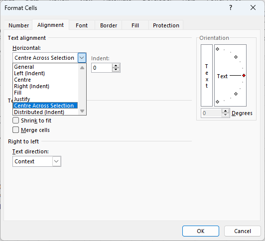
Format this cell with a large font for easy visibility. Apply a font colour if you like. Mine is teal.
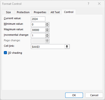
Add a spin button from the Developer tab to easily change the year.
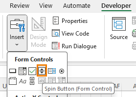
Right-click the spin button > Format Control. Link this button to the cell with the year value.
Add a heading and underline for the header section:
3. Create the Calendar Layout:
Enter the names of the months across four columns and three rows.
Format these month labels with a stylish font and teal colour for a cohesive look.
Insert the days of the week under each month name. Your calendar will start on Sunday, but if you prefer Monday, we'll cover that change later.
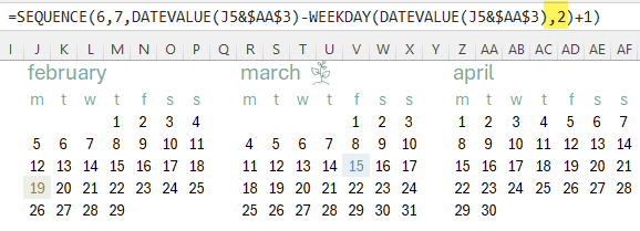
Generate the Dates
Dynamic Date Formula: use the SEQUENCE function to fill in the dates for each month dynamically. We'll use it to create a grid (6 rows x 7 columns) of dates that automatically adjusts based on the month and year.
The formula is:
=SEQUENCE(6,7, DATEVALUE(B5&$AA$3) -WEEKDAY( DATEVALUE(B5&$AA$3) ) +1)
Let's break it down:
1. SEQUENCE(6,7, ...):
Generates a sequence of numbers in a 6x7 grid (6 rows, 7 columns).
The third argument (start) of the SEQUENCE function is the starting date. We'll use DATEVALUE to calculate the date based on the month and year:
2. DATEVALUE(B5&$AA$3)
B5: contains the month name (e.g., "january").
$AA$3: contains a year (e.g., "2024").
B5&$AA$3: concatenates the values in B5 and AA3 to form a text string like "january2024".
DATEVALUE(B5&$AA$3):Converts the text "january2024" into a date. By default, it will return the first day of the month (e.g., "2024-01-01").
3. WEEKDAY(DATEVALUE(B5&$AA$3))
The WEEKDAY function returns the day of the week for a given date, where Sunday is 1, Monday is 2, and so on.
WEEKDAY(DATEVALUE(B5&$AA$3)):Calculates the weekday of the first day of the month. For example, if DATEVALUE(B5&$AA$3) returns "2024-01-01" (a Monday), then WEEKDAY would return 2.
4. DATEVALUE(B5&$AA$3)-WEEKDAY(DATEVALUE(B5&$AA$3))+1
This part calculates the date of the last Sunday before (or on) the first day of the month.
+1 adjusts the result to ensure it starts from the correct Sunday.
5. Format Dates
Apply a custom number format that only displays the day portion of the date:
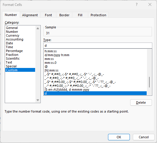
Centre the days, in their cells.
Copy and Paste: Once January's dates are generated and formatted, copy them across to the remaining months.
Conditionally Format Dates
To make your calendar truly dynamic, you'll want to add some conditional formatting to highlight key dates in your date tables.
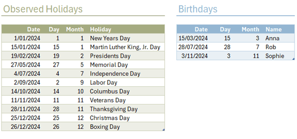
1. Highlight Important Dates:
On a separate sheet, create tables for holidays, birthdays, and other significant dates.
I have two date tables, one for holidays and one for birthdays, but you can add more date tables as required.
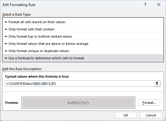
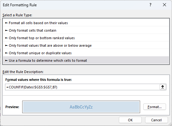
Apply the Conditional Format: Select the cells in the calendar to format > Home tab > Conditional Format > New Rule.
Use COUNTIF formulas in the conditional formatting rules to match these dates and apply unique colors for each category (e.g., taupe for holidays, blue for birthdays).
The holidays rule is:
The birthdays rule is:
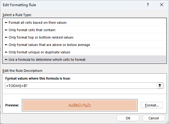
And the rule to highlight today's date is:
2. Hide Overflow Dates:
To keep your calendar clean, you can hide dates that don't belong to the current month. This involves setting up additional conditional formatting rules that compare the month of each date to the month in the header.
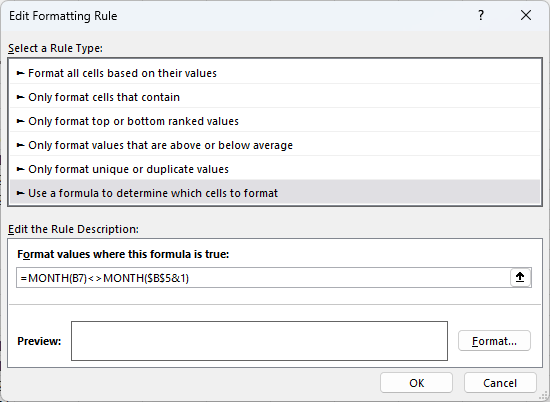
Format the cells with white font and white fill to hide the dates returned by the SEQUENCE formula that don't match the month name in the header.
Adding Personal Touches
Finally, to make your calendar more visually appealing:
Add Icons:
Use icons from the Insert tab to represent different seasons or events.
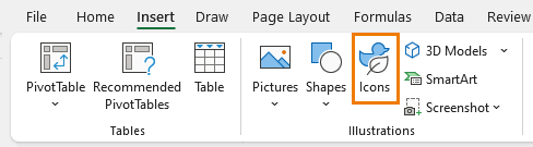
Resize and position them to enhance the overall look of your calendar.
Start on Monday:
If you prefer your week to start on Monday, simply modify the WEEKDAY function in your formula to make use of the 'return_type' argument in WEEKDAY. Inserting '2' in this argument will start the week numbers on Monday instead of the default which is Sunday:
Also adjust the week day headers to start on Monday.
Conditional Formatting Mastery
Creating a dynamic Excel calendar might seem complex at first, but once you get the hang of it, the possibilities are endless. Not only does it help you stay organized, but it also adds a touch of personalization to your planning.
However, because the logic behind the conditional formats is hidden, understanding how to create the necessary formulas can be challenging. But once you get the hang of it, the possibilities are almost limitless.
In my comprehensive tutorial on Conditional Formatting with Formulas, I'll take you behind the scenes to show you how Excel uses conditional formatting formulas, so you can fully tap into its potential.
By the end, you'll be ready to apply these techniques to any Excel project.

Hello Mynda!
Your calendar is amazing and such a great find, thank you!
Is there a way to adapt your template for it to have begin and end dates for each event in the “Dates” tab that, in the “Calendar” tab, will color all the days between and including those begin and end dates? To be noted, for one-day events, the begin and end dates would be the same.
Thanks!
Great to hear, Nat. Yes, you can modify the conditional formatting rule to format a range of dates. I do this in my project management dashboard.
Hi.
Is there anyway to add content to the ‘day’ cells without crashing the sequence formular?
I would love to use this as a work calandar to log hours spent on different projects.
Thanks.
No, sorry. You’d have to insert blank rows after each week of dates for your notes, but that would mean a separate SEQUENCE formula for each row.
Is there a way that a blank row could be eliminated? For example, February and March 2026 both start on a Sunday and the first row of my calendar for both months is completely blank and the month is starting on line 2. I would like to eliminate the blank row 1 and have the month start on that line. Any tips?
Hi Alexis,
I’m currently on vacation, but we have a support forum you can use to get answers to your questions: please post your question on our Excel forum and for a speedy response also upload your Excel file.
Mynda
I love this… just wondering if there is any way to have some kind of pop-up that shows which date(s) are listed on holidays/birthdays when you hover over a date? I’m happy to use VBA if necessary!
You’d have to use VBA to implement popups, maybe using the old-style comments which are now called Notes.
Good day
I am struggling to add more Birthdays, please share or advice how to do so.
Thanks
Hi Tiaki, it should be as simple as selecting the next available cell below the current birthdays table and adding a new one. If you’re still stuck, please post your question on our Excel forum where you can also upload a sample file and we can help you further.
There is one fundamental problem I see in this and that relates to dynamic dates that change each year. In your example spreadsheet Thanksgiving changes to be a Friday in 2025 then a Saturday in 2026, etc so its a static date (always 28 Nov) rather dynamic to always be the 4th Thursday of November. Same issue with things like Easter that changes date and even month every year. Is there a way to get a dynamic date linked somehow into the dates sheet so the dates update as the year changes?
Hi Eric, It sounds like you didn’t download my template, as you’ll see my dates are dynamic, so Thanksgiving always lands on the 28th etc. I didn’t cover that in detail in the video in the interest of time, but the file download link is in the post above where you can see the formulas.
The problem with the calendar is that certain holidays do not fall on fixed dates, but on fixed days during the month. For instance:
Martin Luther King Day is always the 3rd Monday in Jan.
Presidents Days is always the 3rd Monday in Feb.
Columbus day is the 2nd Monday in Oct.
Labour Day is always the 1st Monday in Sept.
Thanksgiving is always the 4th Thursday in Nov.
Ah, yes. I see what you mean. You can still build these dates with formulas. To see how it’s done, go to the File tab > New and search for “Any year calendar with holidays” and you’ll find a template with formulas for those dates.
or power query a date site (i.e. calendar-365.com/holidays/2026.html) for holidays and make that your table?
Lets say we have 4 collegues in office.
We all set ourselves a date(s) for holiday, every month one day or two….
How to add this date to the annual calendar? because i get how you set holidays as this are same dates every year, but how to add this specific dates in the calendar? i will also later set the coloring for each of us, so we will know who is who in the calendar 🙂
You can add a condition to your conditional format to also check that the names match the name listed in the holiday table, so the format is applied to the relevant person.
Hi Mynda, this helped me a lot! thank you! however i’m facing an issue, it seems like the dates are highlighted on other years, I’m unsure what i’m doing wrong, please help me. Thank you in advance
Download my example file and you can see in the list of dates table how I generate them with a formula that picks up the chosen year.
Is there a way to adapt this for school year, to show September to August?
Yes, just rearrange the months accordingly and add a year to the reference to cell AA3 (AA3+1) for Jan to Aug months.
Is there a formal to use in the Conditional Formatting if I still want to use two different colors for holidays and birthday but the list is all in one?
Hi Ray,
You’d have to add a column to tag the dates as holiday or birthday etc. so you can differentiate them in the conditional format.
Mynda
Hi Mynda
Is there away to conditionally format cells if there are two occurrences on the same date? I have a list of Birthdays and a list of Wedd Anniversaries with conditional formatting for each list. When there is a Bday and a Wedd Anniversary on the same day only one shows
Hi Colin,
Kind of. You could write 3 rules, one for birthdays (say with a green cell fill), one for anniversaries (Red cell border) and one for where both are true (red border with green fill).
You’d have to set the rules in the correct order so the last rule is where both are true.
Mynda
How would you write that rule if both were true?
I love the calendar. I followed the tutorial my calendar for the current year works great but when I use the spinner to change years any non-current year is blank. Any suggestions on how to fix or what I may have gotten wrong?
Hi Amy,
Please post your question on our Excel forum where you can also upload a sample file and we can help you further.
Mynda
Formula in Conditional formatting
=MONTH(B7)MONTH($B$5&1)
Wont work for public holidays, for instance May 1st will show twice, in April on hidden days (coloured white) and in May.
Any solution to this?
Still waiting to see how will Today() formula work, in regards to repeating the same on dates that are coloured white.
PS Downloaded the file, when I changed year, it all went with #VALUE! errors.
The MONTH formula in the conditional formatting rules is hiding the second instance of May 1st from April’s calendar even with the public holiday formatting applied. You must put this rule at the top, so that it overrides the public holiday rule. If you’re getting #VALUE errors, then I’d say you have an older version of Excel that doesn’t have the SEQUENCE function.
#VALUE may depends on Country. In Germany I give into the Cells the german Monthnames for the DATVALUE() and then it works.
I had the same problem. I solved it by changing the names of the months to my own language.
Glad to hear you figured it out, Jef.
Hi,
The formular =SEQUENCE(6;7;DATEVALUE(B5&$AA$3)-WEEKDAY(DATEVALUE(B5&$AA$3))+1) doesn’t work for me (in Belgium).
How can this be?
I’m receiving a Value# error message.
Hard to say without seeing your file and what is in cells B5 & AA3. Please post your question on our Excel forum where you can also upload a sample file and we can help you further.
Instead of january, february and so on please set in the headers the belgian monthnames in your language, this could help.
Great tutorial. I’d like to create an additional table, in the “Dates” sheet, with this table being fillable and editable, so that I could continue to add events as the year goes. I’d probably name it “Work Related” or similar, and add dates to that particular table as needed, and the hope would be that the dates would show on the annual calendar.
I’m a fairly novice Excel user, although I can follow tutorials. How do I create a new table, in the “Dates” sheet, with this particular table titled “Work Related,” with the color green, and have it editable/fillable to add pertinent dates as they come, and have those dates show in the annual calendar, similar to the “Observed Holidays” and “Birthdays” tables in the example?
Hi Adam,
Great to hear you can make use of this dynamic calendar. See this tutorial on how to insert Tables, name them and format them.
Then follow the video steps above to add the conditional format for the Work Related table. Note: in the COUNTIF formula, select rows past the current bottom of the table to allow for more rows to be added, so they’re automatically included in the format.
If you get stuck, please post your question on our Excel forum where you can also upload a sample file and we can help you further.
Mynda
Thanks for developing and sharing the content, much appreciated! Can you please include the following as well.
Please consider including to make it dynamic if feasible:
1. Week numbers (in column of every week)
2. To add a to-do list for a week / copy from outlook calendar
3. Hover the cursor/ pointer on date to see the holiday type/birthday person name/to-do list
Great ideas, Amit. You’re welcome to modify it to include those features. You can add the week numbers with the WEEKDAY function in a column to the left of each month’s dates.
Mynda:
This is neat idea! A couple questions:
I added a Dec 12th birthday to the birthday table for Ralph, by adding a new row (8) to the table and found that the date it displayed in cell G8 had the month and day reversed. The original entries displayed correctly using my date format (USA) but the added row did not, even though I confirmed that the formula in G8 was the same as the one in the row above, =DATE(‘Annual Calendar’!$AA$3,[@Month],[@Day]). Not sure what’s going on.
With the above added row, neither 12/7 nor 7/12 appeared on the annual calendar, which I found was because the conditional formatting is tied to a hard range on the Dates sheet, thereby losing the ability to reference the entire range of the table for the conditional formatting. Is there a way around this? It would nice to be able to use the expanding range capabilities of Excel tables for this.
I always enjoy your emails and blogs. Thanks for doing this.
Hi Glenn,
I suspect the date being reversed is just a regional formatting difference. If you CTRL+1 the cell you’ll probably see on the Number tab that the date format is dd/mm/yyyy. You can simply change it to your regional setting of mm/dd/yyyy.
Conditional Formatting doesn’t recognise table structured references so you can’t make it dynamic as such, however you can simply select more rows in the COUNTIF formula than the table currently has to allow for more rows to be added in the future.
Mynda
What if it’s a different language?
It’s better to change the name of the month to the formula =TEXT(MONTH(1);”mmmm”)
Yes, great idea if you need the language to be dynamic too.