I know you’re probably thinking that everyone knows how to use the SUM function, but I’m willing to bet that most people don’t know all the shortcuts and tricks I’m about to show you. These are SUM function tricks you can use every day, and some also apply to all Excel functions.
Watch the Video

Download Workbook
Enter your email address below to download the sample workbook.

Excel SUM Function Tricks
Trick 1: AutoSum
AutoSum detects the range you want to sum by looking for rows/columns adjacent to the cell you have selected that contain numbers. You’ll find it on the home tab:
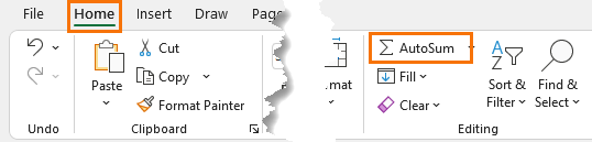
However, I find the keyboard shortcut ALT+= easier to use.
Tip: Select the whole table plus a blank row and column for the sum formulas and ALT+= to automatically enter the SUM formulas for each row and column:
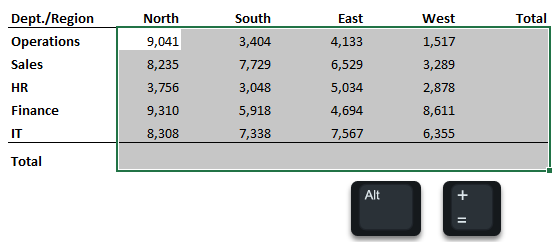
Bonus tip: you can select non-contiguous ranges and press ALT+= to insert multiple AutoSums – see video for demo.
Trick 2: CTRL shortcut for non-contiguous ranges
If you want to sum non-contiguous cells, hold the CTRL key while you select the cells with your mouse to have Excel automatically insert the comma separators for you. This works for other functions too.
Bonus tips not in the video from Bob Umlas - AutoSum Subtotals: To insert a Grand Total for a range of cells containing sub-totals, select the whole range including the cell you want your grand total in > ALT+=
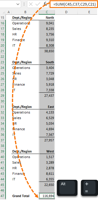
Or simply SUM the entire range and divide by 2 e.g. using the example data above in cell C47 enter this formula:
=SUM(C16:C45)/2
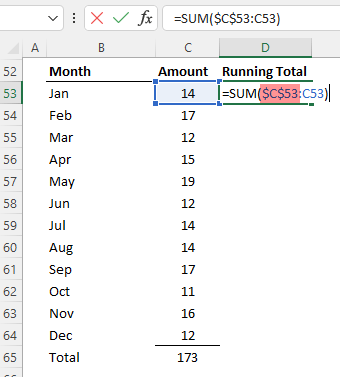
Trick 3: Running Total
To insert a running total reference the first cell in the range, then Absolute reference the first cell in the range before copying the formula down:
Trick 4: SHIFT for 3D ranges
Sum multiple contiguous sheets by selecting the cell on the first sheet and while holding the SHIFT key, select the last sheet in the range:
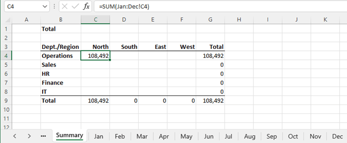
Caution: This will sum all sheets from Jan to Dec. If you drag another sheet inside this range, it will also be included in the sum.
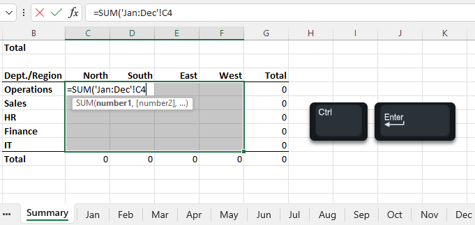
Trick 5: Insert multiple SUM formulas in one go with CTRL+ENTER
Select all the cells you want your SUM formulas in, then enter the first formula and CTRL+ENTER to complete the formula:
If you have a SUM tip or trick, please share it in the comments below.

Question: Is there an easy(!) way to achieve a weighted average?
Hi Linda,
You can use a formula like this: =SUMPRODUCT(values, weights) / SUM(weights)
Mynda
You can have a formula like:
=SUM(A2:D3 (A2,B3,C1,C5,E4,F2,D2))
which forms two ranges and then takes the cells that intersect as the resulting collection of cells to sum. So in the above, cells A2, B3, and D2 from the collection inside the interior brackets are the intersecting cells with the first, more traditional-looking range. So SUM sums up those three cells.
You might think today that such a collection (the interior bracket collection) would need something like VSTACK to collect them into a “real” range or that they would fail to be acted upon. And might wonder just how that VSTACK could be understood by Excel to intersect the first range. You’d be right about the latter concern: it won’t figure it out and will give an error return. And since it isn’t actually needed for direct usage here, why even bother with the extra?
Of course, if you are carefully crafting something with a couple VSTACK/HSTACK ranges (Why? I wonder why? But maybe you have a reason.) then maybe you’d want to figure that out. But simply putting each element into brackets seems… simple… so…
(I’ll grant, maybe the “Why? Just why?” could apply to the use above, but it would’ve solved a couple things for me over the decades, so I’ll stick with it.)
Interesting use case for the space operator, Roy. Thanks for sharing. I covered that many years ago here for anyone who wants an explanation of how it works: Excel Space Operator.
There’s a nice little improvement to something I do. It will ease my life because it will allow one handed input for it letting me not need to switch my left hand back and forth. Yay!
I have a table with 20 or so columns and often need to collect, then later enter, enter several columns of data (not the same in the collecting and entering phases). Presently I have a row above the table in which I do a formula like the following in the index column’s cell and then paste across the columns:
=A43,A65,A96,A122
(Gives a #VALUE! error, but the cell’s output is not of any interest.)
And when I doubleclick the cell for any given column, it selects all the cells in the formula. Then I can collect, or enter, the data desired. Like Ctrl-C to get the values selected and paste them on another sheet in a contiguous block. Or can enter values in the selected cells without navigating down from one to the next. And getting things wrong in either kind of case!
But if I type:
=SUM(
and then click the cells, it will indeed enter the commas for me, freeing my left hand to follow along on the paper records pushing the work. Nice!
I’ll end up with something like:
=SUM(A43,A65,A96,A122
and can then highlight the “SUM(” and delete it leaving the “=A43,A65,A96,A122” I need.
Slick, tightens up the operation, frees my left hand! Win all around.
By the way, the technique need not be non-contiguous cells, nor cells in “order” — they can be ordered any way you like. Have a worksheet displayed form to fill in, but you want to go in a particular order between the entry cells? Or just want to not need to navigate, but rather enter something and press Enter or Tab to move on? Want to guide your boss through his work with it? Lots of other things too. I have some tables that are filled ad hoc, used and then desired to be empty for the next time. The formula will take ranges as well as individual cells, so set up a reusable formula that, when doubleclicked, highlights ALL the cells that can be filled in, then to clear today’s work, doubleclick and press Delete. All wiped clean.
I don’t seem to be able to make it work across sheets, but someday… I’ll suss it out.
But this tricks out the creation of the desired set of cells for the indexing column. Frees my left hand from double duty. Nice!
Wow! That’s a clever trick, Roy. Thanks for sharing. I’m trying it now.
Update…I can’t get SUM to enter the commas unless I hold down CTRL, which means my left hand isn’t free. I also couldn’t get this to work: “And when I doubleclick the cell for any given column, it selects all the cells in the formula. Then I can collect, or enter, the data desired. Like Ctrl-C to get the values selected and paste them on another sheet in a contiguous block. Or can enter values in the selected cells without navigating down from one to the next.”
For the mentioned spreadsheet page, I normally have to enter, or collect, one kind of data at a time, so work with the set of cells for a single column at a time. For instance, one column might have PO #’s. I reserve Row 1 for these formulas, so in the Row 1 cell of the PO column I would create the formula by typing “=”, then clicking the column’s cells for the rows I desire. If I want the rows 3, 7, 10, 11, and 25 in column A, I click them (A3, A7, A10, A11, and A25) in the order desired for however the data needs worked (in this case, almost always exactly in numerical order, of course). So the formula in A1 would be:
=A3,A7,A10,A11,A25
and I cement it with a press of the Enter key.
Then I copy the cell and paste across the table in Row 1 so each column has above its label (so easy to select the right column, not the one next to it) for whatever data I need to enter, or collect. One column might be freight cost, another the date the wire for the shipment of one or more PO’s was placed. Anyway, say column M’s the freight cost column. If I doubleclick the M1 cell, the cells in that column are selected, so M3, M7, M10, M11, and M25. I can now quickly enter the five freight values because pressing Enter (or Tab) after a value moves me to the next cell. I might mention that the cells are sometimes separated up and down by up to a thousand-ish rows, so moving between even three or five can present huge hassles without this.
This works across sheets, so put in the address for cell H459 on Sheet3 and doubleclick and you go to that sheet and cell. Or range. What it will not do, it seems, is select cells on more than a single sheet. If set up for such, it DOES select the cells in the formula, for the sheet you’re on or any other, until it reaches a cell on some other sheet. Then it quits. So
=A1,A80,F2,A3,Sheet3!H34
will select the A1, A80, F2, and A3 cells on the current sheet, but quit, so Sheet3!H34 does not get selected.
Further, if the cell has a file path and name, doubleclicking on it will open that file and the specified cell.
It works on values in working formulas as well. For instance:
=XLOOKUP((F1:F6),B1:B6,K1,K6)
will select F1:F6, B1:B6, K1, and K6 with the first cell of the first range (F1:F6) the current cell, and will navigate in the order shown.
That’s select not show precedents in various colors like when pressing F2.
Used to be, as I believed then and now, like the general Windows problem of the same sort, that the cell you wanted to be current when doubleclicking had to be the last cell listed. So
=A1,A4,G56 would select those cells, but the current cell would G56. Getting A1 to be the current cell and navigating in the same circular order, you needed =A4,G56,A1.
(Windows did the same with file names. Select three files with the mouse to feed into something, say copying them, or better, combining them, and the file you wanted first had to be listed last with the 2nd through 10th listed as 1st through 9th. It no longer has that multi-decade problem and at the same time, this trick no longer needs list the starting current cell last. Yay!)
I find it useful for selecting cells in a “form” as in some on screen display in which one might wish to enter information, but the layout does not lend itself to something orderly, like my mentioned file at the top. Or, say most of the cells are in the screen’s view, but two or three are thousands of rows and hundreds of columns apart. Navigating one to another can be a nightmare. But do this and you pop out to the far off ones and right back to the main area as you press Enter. In any order, back and forth, down and up, etc., that pleases you. On one sheet… Even include after the last far off one, a cell in the nearest corner of the main region (like lower right corner for being in cell DEH204875 and wanting to go back to the main region but have the cell you re-enter it not be the UPPER LEFT corner. You get the right cell (nearest corner to the far off region) and that (in this example) is in the lower right corner with the desired region up and to its left, or in other words, framed on the full monitor screen instead of just that region’s lower right cell in the monitor’s upper left corner. Good, amongst other things, for getting the boss using it, entering or just reading, and not getting all aggravated from having to constantly “get almost there” easily, but then have to futz about to get the main display back on screen.
Cells can be entered more than once.
If one desires a label to display, but to still have the selecting feature, a formula like:
=IF(TRUE(),”Doubleclick Me!”,G3:G9)
will display the Doubleclick Me! message but take you to G3:G9 when the user does that. And more complicated versions can be done. Related: it will accept hashtag addressing. So if M1# has =SEQUENCE(8) in it, doubleclicking selects M1# (M1:M8).
However, if M1 has the same formula, using a range like M1:.M100 (the dot operator) gives you the full M1:M100, not M1:M8. Same with TRIMRANGE.
If you set up multiple ranges, say, to be selected, and they overlap, the overlap will be selected both times, so to speak.
Even things like the intersection operator (=K3:M3 K1:K4) are honored.
Sometimes a complicated setup will see only the first thing selected, so a formula that takes multiple ranges in its construction, like TEXTJOIN which lets you have many ranges listed in it will usually work nicely, but sometimes those (not necessarily using the TEXTJOIN function as the coercion tool) fail. A little hit or miss, and really, not much needed.
The free hand thing… I realized later that it isn’t really free. In MY situation it is… essentially… because the work usually has me (right-handed) using my left hand on the left of the keyboard following along with data to enter and not needing to move to touch the Control key while not doing the SUM trick I wrote this because of required me to either lift it away to be able to type the comma, or to move back and forth, or to do the comma typing with my mouse hand with the same aggravations, or worse. So it isn’t really freed from use, but it can do the use it must without moving about, so in my excited flush I certainly wrongly stated that part. Absolutely.
There are some other limitations as well, but smallish. Lots of uses one CAN put it to are utterly easily done using absolutely simple regular things so why ever bother? Most of the limitations seem to me to fall into those areas, so I haven’t worked on them as much.
An old, old use is to bounce back and forth between cells. Hard to do with, say, HYPERLINK. (Or at least it was hard years ago.) So use the =IF(TRUE,… construction, so like:
=IF(TRUE, “f”, D18)
The “f” could be a formula produced result, not just a number or text, but it can’t have a range in it! So… usually it’s text, or sometimes a number. Like the Doubleclick Me! technique, so likely going from a title to a title, on different pages, and back again, with no garish navigation cells or buttons disrupting your setup.
Mentioning this way to late, but I believe the difficulty you encountered and mentioned, quoting my paragraph, will turn out to be due to me not expressing the idea very well. Hopefully the above (if the setup here allows this long of a post!!!), will express it more clearly. At least reaching enough clarity for you to work out any cloudiness.
Thanks for clarifying, Roy. I’ll try and get some time to work through it.
It has been a long time since I used MC excel. I’ve been retired many years and I haven’t had the need to do formulas for bookkeeping and other documents. I am trying to make an Estate checkbook for my son, that I need to keep an record of incoming monetary amounts and Debits going out and balance. I have tried several formulas that I remember but its not working for me. Is there any temp plate or an formula that you could email me?
Thank you for your help.
Jan Smith
Hi Jan,
I don’t have a template as such, but you might find these tutorials on running totals helpful:
Running Total Formula – not Excel Tables
Running Total Formula – for Excel Tables
You might also find this tutorial on my personal finance dashboard relevant for the reporting.
Mynda
Hi
Please assist me with a countifs formulae
STATUS No of Quotes Value of Quotes
Accepted 4 0
Pending 3 0
ReQuote 1 0
Cancelled 2 0
Total Quotes Issued 10
QUOTE NO DATE CUSTOMER VALUE STATUS
160285 2022-06-10 Unilever R 2 500.00 Accepted
160286 2022-06-11 Sab R 1 680.00 Accepted
160287 2022-06-12 Colgate R 1 120.00 Pending
160288 2022-06-14 Cipla R 3 600.00 ReQuote
160289 2022-06-20 Unilever R 850.00 Cancelled
160290 2022-06-21 Cipla R 925.00 Pending
160291 2022-06-22 Sab R 865.00 Cancelled
160292 2022-06-24 Unilever R 340.00 Accepted
160293 2022-06-24 Unilever R 2 800.00 Pending
160294 2022-06-25 Unilever R 1 468.00 Accepted
Hi Johnny,
Please see this COUNTIFS tutorial. If you get stuck please post your question on our Excel forum where you can also upload a sample file and we can help you further.
This is great!!
Can I access the workbook to practice?
Glad you liked it, Brian. Please see the link to the workbook in the post above which I’ve just added.
Everything else
I will definitely add ALT+= to my list, thanks!
May not be as fast as keyboard shortcuts, but the Quick Analysis toolbar can add not only SUM, but AVERAGE, COUNT, % TOTAL and RUNNING TOTAL to rows or columns. Also, if you are just interested in getting an idea of those numbers without actually adding the formulas, it gives you a preview of the result. Just highlight the range with your numbers and click the Quick Analysis icon that pops up on the lower right of your selection.
Great post as usual, thanks again!
Great to hear, Ben! Thanks for sharing your tips too.
Thanks so much Mynda for another great & clear how to!
Here are some other useful tricks:
Example 1: Summarize absolute values
{=SUM(ABS(A1:A4))} – this is an array formula; the curly braces don’t need to be manually typed, as they are automatically inserted by using CTRL+SHIFT+ENTER
Example 2: Summarize the last 10 values in a list (cell A1 is header)
=SUM(OFFSET(A1,ROWS($A$2:$A$25),0,-10))
Example 3: Summarize intersection of ranges
=SUM(B2:F6 D4:H8)
Example 4: Summarize only the integer part of the numbers from a list
{=SUM(TRUNC(A1:A4))} – this is an array formula (see previous note)
Example 5: Summarize Top 5 numbers from a list
{=SUM(LARGE(A1:A10,{1,2,3,4,5}))} – this is an array formula (see previous note)
or
{=SUM(LARGE(A1:A10,ROW(INDIRECT(“1:5”))))} – this is an array formula (see previous note)
Example 6: Summarize the digits of a number
{=SUM(1*MID(A1,ROW(INDIRECT(“1:”&LEN(A1))),1))} – this is an array formula (see previous note)
Thanks so much for sharing, Andrei!