5 Ways to Link Data in Excel and Automatically Sync

Whether you're working with raw inputs, dashboards, reports, or filtered views, manually updating everything is slow, error-prone, and unnecessary. There are multiple smart ways to link data in Excel, whether it's from another sheet or workbook, and sync it automatically.

In this guide, you'll learn 5 methods to extract and reuse your data, so it updates without lifting a finger, plus when to use each one.

Watch the Video

Get the Excel Example File

1. Linked Cells

One of the simplest methods is to link cells directly using formulas:

For the same file:

Just type = then click the source cell.

This pulls in the value from cell A2 on the 'Annual Revenue' sheet. Notice sheet names are followed by an exclamation mark and those with spaces are also wrapped in apostrophes.

For another workbook:

Open both files and type = then click the source cell in the external workbook.

Notice external references are prefixed by the file name wrapped in square brackets. Once the external file is closed, Excel adds the full file path. However, this is where things get risky.

Problems with Linked Cells:

• Empty cells return zero; fix with &"" for text, or custom number formatting (#,##0;-#,##0;) for numbers.
• New rows must be manually included unless you use the Trim Ref Dot Operator (Excel 365 only):

The :. operator trims trailing blank rows automatically.

• External links break easily if the file is moved or renamed.
• Formulas may fail if the external file is closed (e.g. SUMIF won't work).

Use Linked Cells for: quick, low-risk internal links in small files.

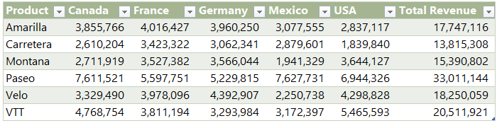
2. Table Structured References

Excel Tables make linking easier and more reliable.

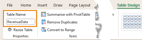
Convert your range to a Table:

Press Ctrl + T, then name the table via the Table Design tab (e.g. RevenueData):

Now you can refer to entire columns with structured references:

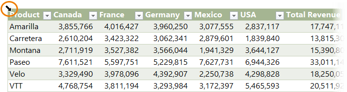
To return the whole table including headers, place your mouse in the top-left corner of the table and click twice (not double click).

Benefits:

• Automatically expands with new rows.
• Changes to the source data are reflected instantly.
• Clean and readable formulas.

Use Tables when: you want dynamic ranges and better formula readability and you don't have access to the new trim ref dot operator.

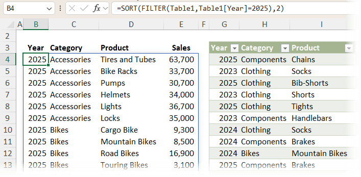
3. FILTER Function

Need to extract data that matches certain criteria? The FILTER function is your best friend.

Example:

This returns only the rows where the Year column equals 2025.

Advantages of FILTER:

• Fully dynamic; updates with your source data.
• Can filter by multiple criteria.
• Easily rearrange or select specific columns.

Use FILTER when: you want to extract specific rows or columns and want instant updates to flow through.

Watch the full FILTER tutorial

4. PivotTables for Full Data Extraction

Think PivotTables are only for summaries? Think again.

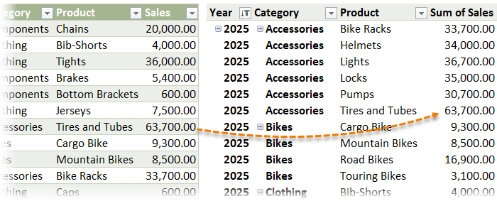
By dragging all text columns to the Row Labels, and value columns to the Values area you can extract every record from your source data; no aggregation required.

Steps:

1. Insert PivotTable from your source range.
2. Drag all attribute fields (Year, Category, Product) into Row Labels.
3. Drag value fields like Sales into the Values area.
4. Set layout to Tabular and repeat item labels (PivotTable Design tab > Report Layout).
5. (Optional) Add Slicers for easy filtering.

Bonus:

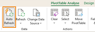
If you're on Excel 365 Beta channel, enable the new Auto-refresh so the PivotTable updates as the source changes.

Use PivotTables when: you want a stable, filterable mirror of your data; great for dashboards and reports.

5. Power Query (Best for External Files)

When working with external files, Power Query is the most reliable method.

Steps:

1. Go to Data > Get Data > From Workbook (or whichever source your data is in)
2. Select the sheet or range you need.
3. Use the Power Query Editor to clean your data, e.g.:
   • Filter rows
   • Remove or rename columns
   • Split or merge columns
   • Aggregate data etc.
4. Load the result:
   • To a table
   • To a PivotTable
   • To the Data Model
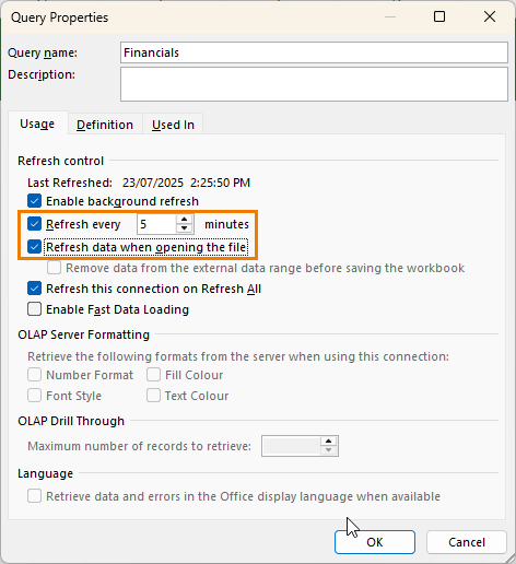
5. Enable auto-refresh:
   • Display the queries and connection pane (Data tab)
   • Right-click the query > Properties
   • Set it to refresh every X minutes
   • Enable refresh on open

Why Power Query is better than formulas:

• Doesn't require the source file to be open.
• Less fragile - renaming or moving files won't break queries.
• Ideal for automating data transformation and cleanup.

Use Power Query when: you're importing, filtering, or transforming data from external sources.

Watch: Automate boring Excel tasks with Power Query

Summary: Which Method Should You Use?

Method	Best For	Excel Version
Linked Cells	Quick, simple links in the same file	All versions
Table References	Auto-expanding, structured data	Excel 2007+ and M365
FILTER Function	Criteria-based extraction	Excel 2021+ and M365
PivotTables	Full or partial data extraction + filtering	All versions
Power Query	External file imports & transformations	Excel 2016+ and M365

Final Thoughts

Automating your data extraction in Excel saves time, reduces errors, and makes your workbooks more scalable. From simple linked cells to powerful tools like Power Query, there's a method for every use case.

Start with Tables and FILTER for quick wins inside the same file.

Use Power Query for anything external, repetitive, or needing cleanup.

Need help mastering these tools?

Check out our Advanced Excel Formulas course for step-by-step guidance and real-world examples.