The other day a member emailed me the following question:
“I created a check book in Excel 2010 and I was able to figure out the running balance which basically adds, subtracts accordingly and it gives me a running balance.
My question is; is there a way to display that running balance (considering it keeps changing rows with each new entry) in another cell?
I am trying to create a cell near the top of the worksheet that also displays my current balance and well as within the worksheet.
Any thoughts?
Steve.”
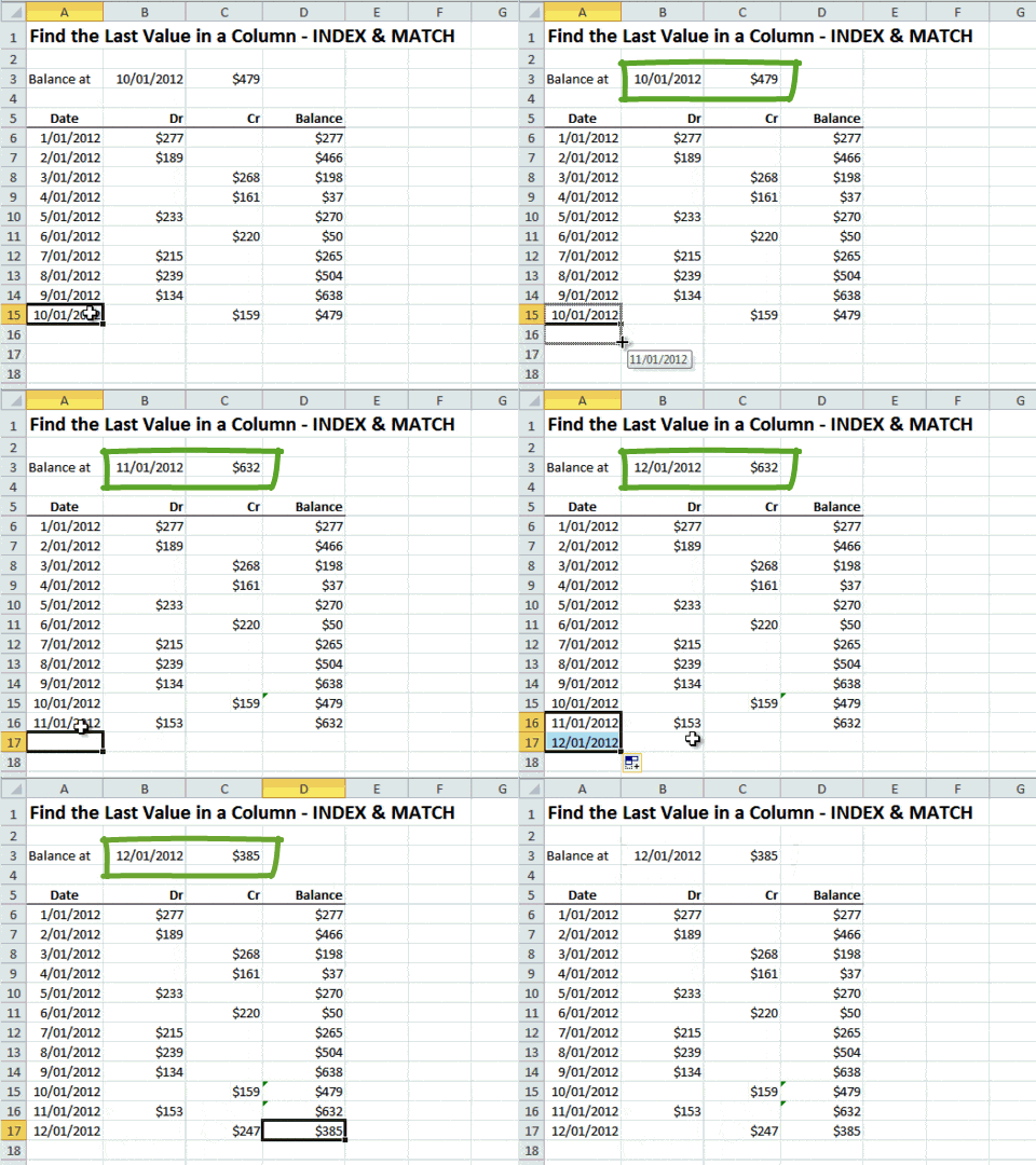
Let's assume Steve has a worksheet something like the example below, and he wants a formula that updates to find the last value in the 'Balance' column, like the one in cell C3:
It's actually quite easy. With some clever use of the INDEX and MATCH functions we can use the following formula:
=INDEX(D6:D500,MATCH(9.99999999999999E+307,D6:D500))
I've also used this formula in cell B3 to get the latest date from column A, like this:
=INDEX(A6:A500,MATCH(9.99999999999999E+307,A6:A500))
You can do the same for a row, just change the cell references to reference a row rather than a column. For example:
=INDEX(C2:X2,MATCH(9.99999999999999E+307,C2:X2))
Finding the Last Text Value
The above formulas work if the data in your range is numeric.
But if it’s text you want to look up then you’ll need this formula:
=INDEX(D1:D500,MATCH(REPT("z",255),D1:D500))
I actually used this technique in my 'toughest Excel challenge ever' but I think it's a great technique to use on its own too.
Thanks for your question, Steve.


Hi Mynda,
I have been using your formula on weekly data for years to find the last value in a col that includes #N/A values. Now I want to find the last three values in that column – so I can calc the change from 1 week to the next. Can your formula be modified to do this?
Jerry
.
Hi Jerry,
If you have 365, you can use the TAKE function to get the last 3 values. If you get stuck, please post your question on our Excel forum where you can also upload a sample file and we can help you further.
Mynda
I have Excel 2010, This seems to work — It gives me values that correspond to the last 3 values in the col.
=INDEX(E10:E1824,MATCH(9.99999999999999E+307,E10:E1824))
=INDEX(E10:E1824,MATCH(9.99999999999999E+307,E10:E1824)-1)
=INDEX(E10:E1824,MATCH(9.99999999999999E+307,E10:E1824)-2)
Jerry
Glad you found a workaround for Excel 2010, Jerry.
Thank you for this useful formular, i’ve solved my problem issue via this technique . It;s really work and helpful.
Best regards,
You’re welcome, Trang 🙂
I was surfing the net in an attempt to understand “LOOKUP(9.99999999999999E+307” when I came across your link. To me what makes this forum special is the lengths you take to explain your answers.
and the extra mile you went in this case to show a similar formula for text.
Thanks a million! 😀
Aw, cheers Martin. Hope to have you back here from time to time. 🙂
Using your Index/Match formula gives me the proper result, but I am running into a problem trying to use that result in a subsequent calculation. I am using the formula =IF(I4-J4+L4=K4,”Good”,”Bad”), where K4 represents the results of the Match Index search. I am getting a “No” result, even when the math indicates it should be a “Yes”. If I type over the Index Match result and enter the same number manually, I get the appropriate “Yes” response. Can you help?
Hi Bob,
Is it possibly a rounding issue? I would increase the number of decimal places displayed by your INDEX/MATCH result and double check the number.
If that’s not the problem you can send me the file and I’ll take a look.
Cheers,
Mynda.
Hello! It took me a while to figure out why this works…might have been helpful to explain that Match searches in ascending order when you omit the match_type argument! 🙂
Hi Shelley,
Thanks for your feedback. I agree the MATCH function arguments could be listed. I’ll add some additional info to the INDEX MATCH tutorial.
To recap; the syntax for the MATCH function is:
=MATCH(lookup_value, lookup_array, [match_type])
Note: when match_type is omitted (which it is in the examples above) it uses the default of 1, which means it will find the largest value that is <= to the lookup_value, but there’s an exception to this rule. Here's an extract from excelbanter.com as to why it works:
In Excel the value 9.99999999999999E+307 is considered the largest value Excel can handle, which is why it is used as the lookup_value.
Arguably you could use another number just so long as it would always be larger than any number in your array.
I hope that helps. For more eye-glazing details read this discussion.
Kind regards,
Mynda.