When you spend days crafting your latest report, the last thing you need are well meaning users messing with your file. In this tutorial I’m going to show you how to use Excel workbook protection which will allow your users to experience the report as you intended. They can:
- Click Slicer buttons
- Refresh data connections
- Select items from drop down lists/data validation
- Click hyperlinks
- But they can’t break it!
Watch the Video

Get the Cheat Sheet
Enter your email address below to download the cheat sheet.

Written Steps for Excel Workbook Protection:
Unlock Cells
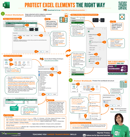
By default, all cells and objects in the workbook are locked. However, this doesn’t come into effect until you protect the sheet via the Review tab of the ribbon:
For most reports and dashboards, you won’t want any cells unlocked, but if you have data validation lists you want your users to interact with, then you’ll want to unlock those cells before protecting the sheet. Likewise for hyperlinks.
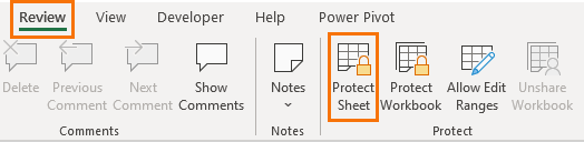
To do this, CTRL+1 to open the Format cells dialog box > Protection tab > deselect the ‘Locked’ box:
Hyperlinks
If you have any cells containing hyperlinks, you’ll need to unlock them before protecting the sheet. However, you don’t need to unprotect objects with associated hyperlinks as these will still be clickable when the sheet is protected.
Allow PivotTable and Slicer Interaction
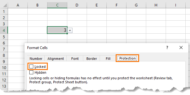
Slicers: Slicers must be unlocked for your users to be able to select items. To do this, select the Slicer (hold SHIFT or CTRL to select multiple Slicers) > CTRL+1 to open the format pane > under Position and Layout check the ‘Disable resizing and moving’ box. This will prevent the pull handles on the Slicer appearing when the Slicer is clicked, and of course as a result, your users can’t move or resize it.
Under Slicer Properties deselect ‘Locked’.
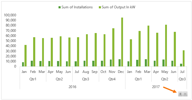
Pivot Charts: If your Pivot Charts have field buttons, like the expand and collapse buttons shown below, that you want your users to interact with then you’ll also need to unprotect the charts. Most of the time your Pivot Charts won’t have any field buttons, so you’ll want to leave them protected.
To unprotect a chart, select the chart border then CTRL+1 to open the formatting pane where you can turn off protection.
Note: regular charts should stay protected.
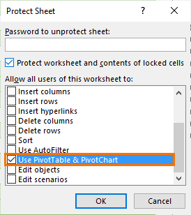
Be sure to check the ‘Use PivotTable & PivotChart’ box so they can be updated when any Expand and Collapse buttons or Slicer buttons are selected:
Form Controls
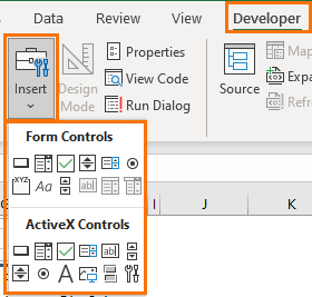
If your reports use Form Controls, like buttons or check boxes available from the Developer tab then there’s no need to unprotect them as they remain interactive when locked.
Hide Formulas
If you have lots of formulas in your dashboard or report that you don’t want users to be able to inspect, be sure to deselect the ‘Select locked cells’ box:
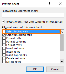
This will prevent users being able to select any locked cells and as a result they cannot see the underlying formulas in the formula bar.
Hide Workings
The only sheet visible in your file should be your dashboard or report. Put your source data, workings and PivotTables on hidden sheets, then set Workbook Protection to prevent users unhiding them.
IMPORTANT: do not also protect your hidden workings sheets as this will prevent refreshing data connections and PivotTables that support your dashboard or report.
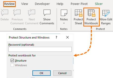
Excel Workbook Protection
Once you have protection set at the cell, object and worksheet level you can set up workbook protection to prevent users unhiding the worksheets that you’ve hidden.
Excel Workbook Protection Caveat
Worksheet and workbook level protection is not intended as a security feature. It simply prevents users from modifying your reports. Don’t rely on it to keep sensitive information private because the password protection can be removed with a range of free tools and techniques available through a simple Google search.
If protecting sensitive data is essential, please consider using Power BI, which has built in security features that allow you to restrict data access to only those with authorisation.
