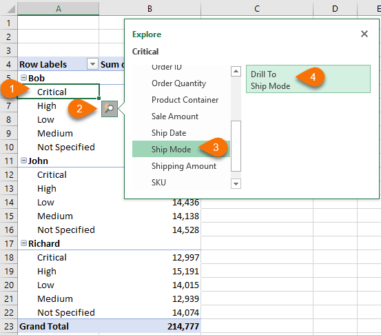
With PivotTable Quick Explore we can filter and drill down in PivotTables and Pivot Charts without the field list exposed. This means our users can customise their reports without needing to know how to build a PivotTable:
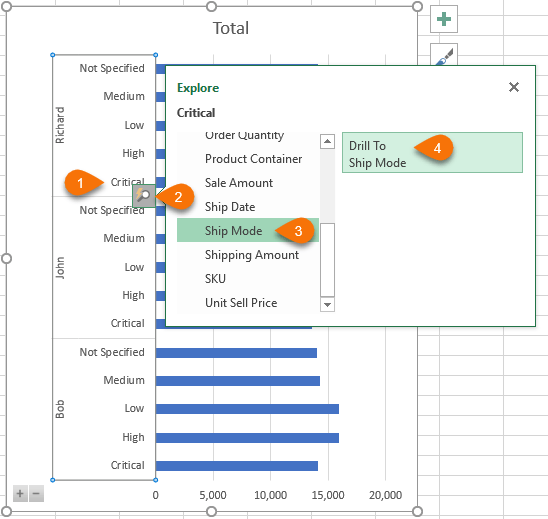
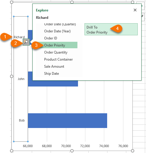
Quick Explore is also available in Pivot Charts:
Note: Applies to Excel 2013 onward for Power Pivot/Data Model or OLAP PivotTables.
Excel PivotTable Quick Explore requires the source data to come from the Data Model (aka Power Pivot), or an OLAP (Online Analytical Processing) cube. In other words, it doesn’t work with regular PivotTables and only works in Excel 2013 onward where Power Pivot is built into Excel, as opposed to an add-in.
Watch the Video

Download the Workbook
Enter your email address below to download the sample workbook.
Building PivotTables for Quick Explore
In the Create PivotTable dialog box (Insert tab > PivotTable), you can either connect to an external data source:
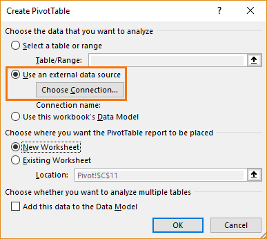
And navigate to your OLAP database, or other relational database like Access.
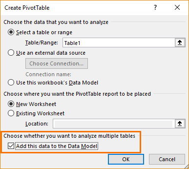
Or if your data is in an Excel Table you can check the box to load it to the Data Model upon creating the PivotTable:
Using Excel PivotTable Quick Explore
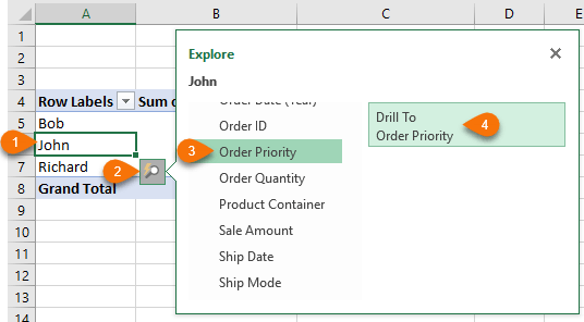
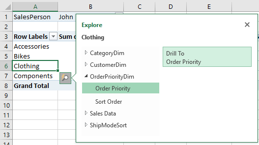
To use Quick Explore, first select a single cell or item in the PivotTable that you want to filter on, then click the magnifying glass, or right-click > Quick Explore. From here you can choose the table and field you want to drill down to.
In the example below notice that I’ve selected John, which will become my filter. Then I want to drill down to the Order Priority field:
And below you can see that John has become the Filter (cell B2) and the row labels contain the Order Priority:
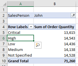
We can continue to drill down further into the data. For example, from here we can filter Order Priority ‘High’ and drill down to the Product Container:
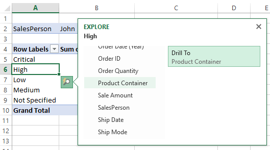
Now we have two filter items; Salesperson ‘John’ and Order Priority ‘High’, with the Product Container in the row labels:
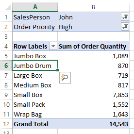
If you have multiple tables in your Data Model/Power Pivot, then those will appear with an expand icon to the left of the table name. Clicking on this will reveal the fields in the table:
So, now that you’ve drilled down you’re probably wondering how you drill back up. Well, there’s no drill up as such, but you can use CTRL+Z or 'Undo' on the Quick Access Toolbar to undo the filter and drill down.
Excel Quick Explore Pivot Charts
Quick Explore works the same in a Pivot Chart, except you select the item in the axis to trigger the Magnifying Glass icon:
Excel PivotTable Quick Explore Things to Note
- The hierarchy can come from the source data or grouped items, like dates etc.
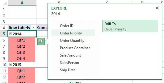
- If you already have a hierarchy in your PivotTable it will be replaced with the field you drill down on.
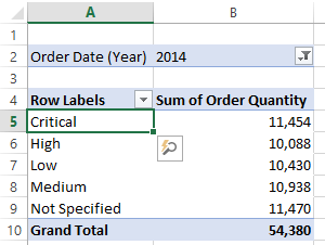
For example, in the PivotTable below I’ve selected 2014 to ‘Explore’ and I’m going to drill down to the Order Priority, which will replace the quarters currently in the row labels:
In the image below, you can see the quarter breakdown has been removed from the PivotTable altogether:
Excel PivotTable Quick Explore Limitations
- Your data needs to be in a hierarchy that supports drilling down. e.g. flat hierarchies or hierarchies that don’t have data on multiple levels are not supported.
- You cannot drill down on named sets.
- Unfortunately, you cannot turn off the Quick Explore pop up icon.
Alternatives to Quick Explore
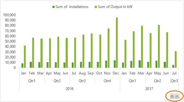
If you want to retain the levels in the hierarchy as you drill down then an option is to use the Expand/Collapse buttons. These are available in Pivot Charts in Excel 2016 onward:


I’m with Jim and Zack,
I’ve never seen this and it does NOT appear in the downloaded example spreadsheet
I’ve had 365 for nearly 2 years now and all data is added to the Data Model
from some of the other comments, perhaps that’s lucky!
jim
Hi Jim,
I’m thinking this is some kind of licensing limitation, however there’s no mention of this restriction in Microsoft’s documentation for Quick Explore.
Mynda
Simply brilliant!
Ever since starting your courses, I have wondered what the magnifying glass icon and other things were.
I have found that the best way to proceed is to just remember the puzzling item and carry on with the work. (A bit like quantum Physics, Copenhagen Flavour: Shut up and keep on calculating!!) now knowing that eventually, all will be made clear.
You must think that I am becoming a bit of a groupie! I have given up looking at other Excel videos – they are either too boring, or the presenter clearly doesn’t really understand the intent of the tool he is droning on about. Technically, they are OK, but they provide no context.
I watched one covering Solver. Yes, they knew how solver worked, but they had clearly never done any Linear Programming at all, and they didn’t know why they were using the tool or why it worked. In fact, it produces correct answers that are useless to the user for quite a wide range of problems. For that, he would need to understand the context and how to fix the unusable results.
Thanks for your kind words, Steven! It’s great to know you find my tutorials helpful 🙂
I’m confused…
I use MS 365 and can’t seem to find Quick Explore in Excel.
I set up a pivot table using your downloaded file and right-clicked, poked and prodded to find the magnifying glass, but to no avail.
Am I missing something?
Hi Jim,
I’m also using 365. I wonder if you haven’t loaded the data to the Data Model?
Mynda
Once you’ve selected Quick Explore and drilled down, are there any ways to go back out without using Ctrl+z? I need to use quick explore to drill down on a table I was given for which I was not given the source data. I then need to copy+paste the resulting tables with the detail I need onto a separate file. However the only way I can find to navigate back to the upper levels is using Ctrl+Z which basically undos the pasting of the table, making my entire task pointless! Does anyone know a work around for this issue?
Hi Joana,
That’s a great question! You’d have to edit the fields in the field list to revert the PivotTable back to its original state. I don’t know of any automatic way other than Undo.
Mynda
To whom it may concern,
The quickexplorer option in excel doesn’t pop up when I click on a pivot table cell. Is there a setting to turn it on?
Thanks
Hi Zack,
Did you add your data to the data model/Power Pivot? Quick Explore is only available for PivotTables that use data from the data model.
Mynda
Is there a way to turn off the Quick Explore pop up. For years, I’ve been annoyed by it in Power Pivot and am dumbfounded that there’s seemingly no way to disable this irritating pop up.
Hi Steve,
No, there doesn’t appear to be any way to turn Quick Explore off. You can suggest it on Excel UserVoice.
Mynda
I just submitted a suggestion on Excel UserVoice. We gotta have a way of turning this thing off. It destroys the table. I completely agree with Steve. Unless you have a pivot table that is completely unadorned in a worksheet with nothing else on it and you didn’t care how it changed (had no one, ever) this thing wreaks havoc!
Yes, it’s annoying I agree.
Once again, you have me download a work book and it does not match up with your instructions.
Like Alan Wyatt, you assume that I know as much as you do and blam, I get led into a brick wall.
The Pivot Table in the workbook I downloaded does not match your instructions
Your Pivot Table has Row Labels of years and quarters, not the salesperson
A waste of my time
Sorry, Ted, the PivotTable in the workbook is in the state of the final example in the tutorial above. You can change it and play around with it to try out different scenarios covered in the post above, all the data is there in the file, you just change the row labels as desired. The tutorial wasn’t intended to teach you how to use a PivotTable, that’s a whole other lesson, I simply included the workbook so you had something you could experiment with.
Mynda