It’s often difficult enough to figure out the correct Excel functions to use, but it’s significantly harder if you also need to translate the function into the language of your localized version of Excel.
Introducing the Excel Functions Translator. It’s a free add-in available for Excel Online, Excel 2013, Excel 2016 for Desktop, Office 365, Excel 2016 for Mac and iPad.
The Excel Functions Translator is the result of a Microsoft Garage project by Martin Ørsted and Vadym Khondar who worked on it in their spare time.
It translates some 800 functions into Excel’s 80 localised languages. The add in is currently available in 15 languages; English, Danish, German, Spanish, French, Italian, Japanese, Korean, Dutch, Portuguese Brazilian, Russian, Swedish, Turkish, Chinese Traditional and Chinese Complex Script.
The Excel Functions Translator will:
- Enable users to easily translate full formulas to their native language. So now when you find a formula online you can use the translator to convert it to your localized language and syntax.
- Enable users who know Excel's English functions to become productive in localized Excel versions.
- Provide an efficient way to search for any part of a function's name in both languages selected.
It displays a scrollable, and categorized list of English functions, and their corresponding localized functions.
You can also give feedback to Microsoft on the function translation quality and on a specific function in a specific language.
Installing the Excel Functions Translator
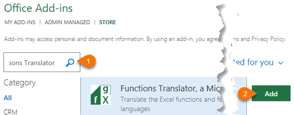
The Excel Functions Translator is installed from within Excel. Go to the Insert tab > Store:

Note: The add-in requires an internet connection to work.
In the search field type ‘Excel Functions Translator’ and then click the ‘Add’ button:
In Excel 2016 the Excel Functions Translator add-in creates two buttons in the far right of the Home tab:

You may need to restart Excel to complete the install.
Click the Translator icon to launch the task pane.
Select the Gear icon in the bottom right of the task pane to set the languages (note: you can only work with one pair of languages at a time):
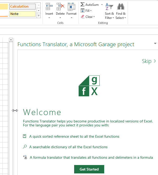
Note: In Excel 2013 and iPad it automatically opens a task pane in the right-hand side of the workbook once installed. Click ‘Get Started’ to set your languages:
By default, the From language will be English and the To language will be your Excel Install language if your install language is one of the languages available in the Functions Translator.
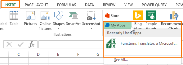
Because there are no icons on the Home tab in Excel 2013 and Excel for iPad, to reopen it go to the Insert tab > My Apps:
Using the Excel Functions Translator
There are 3 tools: Reference, Dictionary and Translator.
The Reference pane gives you a list of functions in your chosen languages. You can use the drop down (1) to choose the Function Category and change the sort order (2):
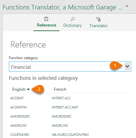
- To sort by the other language, in my case French, simply click on ‘French’. Click ‘English’ to switch back.
- Hover over a function to see a tooltip containing the function description. Note: these are in English only. Localized descriptions are available in the Formulas tab of your localized version of Excel.
- Click on a function name to navigate to the Dictionary pane.
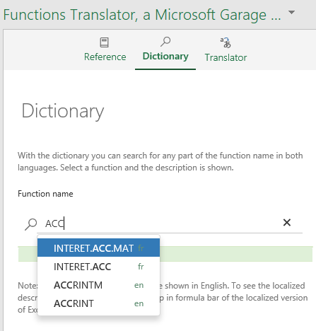
The Dictionary pane enables you to search for a function. As you enter the name you’re presented with a filtered list of functions that contain your search term. Notice the language is noted in green to the right of the function name:
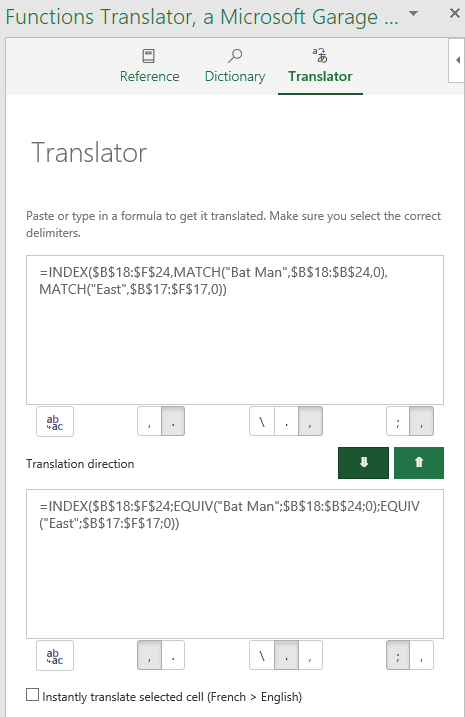
Simply paste the formula you want translated into the top box and click the green down arrow to translate it. Et voila:
Delimiters
The delimiters are set automatically and the shaded delimiter below the formula box indicates the one selected for the language above. You can change the selected delimiter by clicking on the one you want.
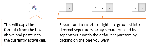
Array separator is specific to Array formulas.
List separator, for English, the decimal separator is normally a period, and the list delimiter is a comma. For some European languages, the decimal separator is a comma, and the list delimiter therefore must be something else, namely a semi-colon.
Instantly Translate Selected Cell
The Instantly translate selected cell option on the Translator tab will attempt to translate the formula in any cell that you select. It will input the formula from the selected cell into the bottom To language box, and instantly paste a translation in the From language box.
To activate it check the box ‘Instantly translate selected cell…’ at the bottom of the pane:

Behind Excel Functions Translator
Learn more about the team behind the Excel Functions Translator and their story.
Please Share
If you liked this please click the buttons below to share.


How do you open it up after it has been added to excel?? I added to excel and used it. But after I closed excel and then open it back up, I can not figure out how access the Functions Translator tool from the menu. do you have to do INSERT> Store > Functions Translator every single time?
Hi TJ,
What version of excel are you using?
As it says in the article, try this:
Because there are no icons on the Home tab in Excel 2013 and Excel for iPad, to reopen it go to the Insert tab > My Apps.
Hi,
I’m getting the following error for this Excel Functions Translator Add-In: https://imgur.com/I73oujX
After clicking on “See Details” button, I get: https://imgur.com/PFQeZC9
Could you please check what’s wrong?
Thanks in advance!
Hi Percy,
That’s typical! I’m not an IE expert but the first message tells you what’s wrong, so now you just need to upgrade Internet Explorer. I’d just do a search on Google for ‘Update Internet Explorer’ and look for the instructions.
Mynda
=VLOOKUP($C7,’Sales Tab’!$F:$CF,’Sales Tab’!AW$7,0), when im puting the formula its taking the value from the AX cell, how?
Hi,
Your formula says:
“Look for C7 value in column F of range F:CF and return the value from column number found in cell AW7”
You have to check what number you have in AW7. Keep in mind that you cannot use cell column number. The column number for VLOOKUP starts from 1, no matter what range you use. In your case, you’re using range F:CF, F is column 1, G is column 2 and so on. If you want column J, you cannot use 10, because column J is column 5 in F:CF range.
Use INDEX MATCH, it’s less confusing:
=INDEX(Z1:Z100, MATCH(C7,F1:F1000,0))
In this example, we clearly indicate column Z to take data from.
The 3rd argument is a number that represents the column number in your range that you want returned. My guess is cell AW7 contains the number 45, which is why the value in column AX is being returned. i.e. because it’s the 45th column in the range F:CF.
More on how the VLOOKUP function works here.
Mynda
Mynda