I have been using Power Query for a little over year doing basic cleanup and merging of data for reports. I am treading new territory with replacing index and match in Power Query, which I know are not function in PQ.
The below formula is used cell D1 thru D5. The same formula is used in cells E2:E5. If the list code and AST1 have a match on the Rep Table, then it will show the Rep Table Location as shown in cell D4. If there is no match, BLANK1 or BLANK2 will show as shown in cells D2:D3 and E2:E3.
=IFERROR(INDEX('REP TABLE'!$F$2:$F$3577,MATCH(1,(Formula!K2='REP TABLE'!$B$2:$B$3577)*(Formula!A2='REP TABLE'!$D$2:$D$3577),0)),"BLANK1")
The attached file, T-Sample, is a small example of what I am working with. The only data not included on this sheet is sales information. I have tried to create some type of helper column with concatenating the salesrep & list code on the Rep Table tab, but I run into an issue with one to many and my numbers get skewed.
Your help is much appreciated! If you need anything additional, please let me know.
Kind regards,
Alicia
Hi Alicia,
You have here a good tutorial describing exactly your case:
https://www.myonlinetraininghub.com/excel-power-query-vlookup
Hi Catalin,
Thank you for the reply. The link for the tutorial took me back to my original post. Can you please send me the tutorial link for my case?
Thank you!
Sorry, fixed the link in the previous post.
The equivalent of Index-Match or VLOOKUP in Power Query is the Merge operation, it's much stronger and flexible than a formula, you can use more than 1 key columns to identify a record.
No problem. When I use the Merge operation on my file, I am running into issues of the sales showing the same for each row as well as the same reps. I was hoping there may have been another way to do this.
Please share more details, an example of your wrong attempts will help.
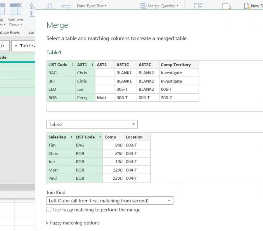
In Merge settings, you can associate more columns as keys, in the attached example I used Rep and Code columns. First table should be sales, second should be Rep Table, Left Outer join type.
Is this what you are looking for?
I created a new sample file with more details and the issue I am experiencing when using the merge operation. When I merge the AST1 on the Sales Query and SalesRep on the Rep Query, remove the columns I do not need to only show the Rep Location, you'll see the duplicate sales for 20 and 21.
I will also need to lookup the Rep Location for AST2 and AST3, but based on the merge operation, it will only duplicate the sales. See attached file.
That's what I mentioned above: you have to merge based on more column keys, as I did in the previous message sample file. I used Rep AND Code columns as keys that identifies a UNIQUE entry in Rep table. If you use only Rep, then it will find more than 1 match in the rep table, all matches will be returned.
Your merge formula:
= Table.NestedJoin(#"Changed Type1", {"AST.1"}, Rep, {"SalesRep"}, "Rep", JoinKind.LeftOuter)
Correct formula, with 2 columns as keys:
= Table.NestedJoin(#"Changed Type1", {"AST.1", "MFG"}, Rep, {"SalesRep", "MFG"}, "Rep", JoinKind.LeftOuter)
See image attached for a correct key mapping, a unique entry in Rep table is identified by 2 columns: AST.1 and MFG (LIST Code), not just Rep.
Also, please follow the tutorial provided, if you don't know how to map multiple columns for merging.
An excel Index-Match combination returns ONLY the first match found, but in PQ, if there are more than 1 matches, all matches will be returned, causing duplicate rows.
If you look at the merged step column before expanding the merge results, you will see that the table contains multiple rows. It is possible to keep only the first row, if you don't want to use multiple merge keys, but it's not right.

Thank you. Now that the merge was done for AST.1, I need to do the same thing for AST.2 and AST.3. When I do the merge for AST.2, my results are null. Is there another way to use that function again to produce the same results showing the Rep Location?
You have to take a closer look at the source data, if the results are not as expected.
If you look at AST.2 column, the names in that column have a space or 2 before the name, it obviously needs some cleaning before merge.
Thank you so much for your help! I was able to get the space before the name cleaned up and everything populated like I needed it.
In Excel I used the IF function to determine the actual location of the sale. My formula in Excel was:
=IF(M5=N5,M5,IF(AND(M5="BLANK1",N5="BLANK2"),"Investigate",IF(AND(M5<>"BLANK1",N5="BLANK2"),M5,IF(AND(M5<>"BLANK1",N5<>"BLANK2",M5<>N5),"300-Corporate",IF(AND(M5="BLANK1",N5<>"BLANK2"),N5,"ERROR")))))
If I add a conditional column in PQ, how can I rewrite the above formula to bring back the actual location of the sale?
If AST1, AST2 and AST3 are Blank, then I need to investigate.
If AST1 has a territory and AST2 and AST3 are blank, return the territory for AST1.
If AST1 is Blank and AST2 has a territory and AST3 is blank, return the territory for AST2.
If AST1, AST2, AST3 has different territories, return 300C.
Hi Alicia,
You have to use column references instead of cell references:
ActualLocation= if [AST.1]=[AST.2] then [AST.1] else if ([AST.1] ="BLANK1" and [AST.2]="BLANK2") then "Investigate" else ....
You have a tutorial here: https://www.myonlinetraininghub.com/power-query-if-statements
