Hi Anders,

That's odd, but then so is the starting point of the vertical axis.

Can you please share your file, or if it contains confidential information please provide a cleaned sample file so we can see the error and all of the contributing factors. There's not much I can tell from the screenshot, other than it clearly looks wrong 🙂

Thanks,

Mynda

Hello,

I have created an example file containing the data for showing this problem.

As you can see in the example file the data value is showing correct if I choose to not to format it, but the number series alone does not tell any good information so I format the data to d "days" hh "hours" mm "minutes". That works fine in the table, but not in the chart.

Either it is a bug or there is a solution for this behaviour.

Br,
Anders Sehlstedt

Hi Anders,

Thanks for sharing the file. There appears to be a limitation on PivotTables displaying day duration with hours and minutes in the one format.

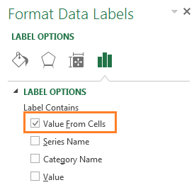
You can either display cumulative hours and minutes ([h] "Hours" mm "Minutes"), or if you have Excel 2013 or 2016 then you can use the 'Show Values From Cells' in your labels and with some reformatting of your PivotTable you can simply reference the PivotTable cells for the labels.

The attached file has both options.

Mynda

Hello,

Thank you Mynda. Yes, by skipping the days in the formatting and only have hours and minutes I get correct values in the chart, but it is a huge difference to read the value as 53 hours and 33 minutes compared to read it as 2 days 5 hours and 33 minutes.

Perhaps this "error" is fixed in later updates, it is after all showing correct in the table.

Using the "Value from Cells" option is not an option for me, as the table is dynamic and grows and shrinks in number of rows. To get correct labels using this option you need a fixed table. At least to my understanding. I will however play around and test this option a bit more, as I normally avoid using this option I am not that familiar with what you can and can't do with it.

I appreciate that you have taken your time to check this out and as you state, there seems to be a limitiation in at least the PivotCharts displaying day duration.

Br,
Anders

Hi Anders,

I agree it's not an ideal workaround. I've asked my MVP community and raised it with Microsoft. I'll let you know if I get a helpful response.

Mynda

Hi Anders,

Fellow Excel MVP, Jon Peltier, discovered that regular charts correctly display the custom day format in both the axis and labels.

So, I recommend you use a regular chart instead of a PivotChart. You can still use your PivotTable as the source data by setting up dynamic named ranges to pick up the PivotTable data, as described here: https://www.myonlinetraininghub.com/create-regular-excel-charts-from-pivottables

Mynda

Hello Mynda,

Thank you for the updates. Please also send my thanks to Jon.

It works very nice with a regular chart combined with dynamic named ranges. Not only have I now a good, if not even a great workaround for this issue, I have also learned how to create a dynamic named range and using Index function in a way I didn't expect it could be used.

Let's also hope that this formatting issue with PivotCharts gets resolved in the near future. When I for example opened the workbook in Excel for Mac (O365) it showed correct formatted values.

Br,
Anders

Will do 🙂

Typical that for once there's something Excel for Windows won't do, that the Mac will!

Glad you liked the INDEX solution for dynamic named ranges. You obviously haven't come across that tutorial in the dashboard course yet.

Ha ha, you got me there.

I work either with tables or PivotTables in Excel, so I usually don't need to use named ranges. But as this issue has shown, even so it is usable to use named ranges. So I will definitly re-check the lesson 5 sessions.