Excel has invisible rules; quiet principles that shape how every formula works. Once you understand them, you start seeing patterns everywhere. Suddenly, your formulas just work. They’re faster, cleaner, and easier to debug.
In this guide, you’ll learn 5 hidden Excel formula rules the pros use daily. These rules will help you write formulas that last, not just formulas that work once.
Table of Contents
- Watch the Hidden Excel Formula Rules Video
- Get the Example File – Practice or use it as a reference guide.
- Rule 1: Build for Humans, Not Just Excel
- Rule 2: Boolean Logic – The Shortcut Pros Use Instead of IF
- Rule 3: Use Invisible Helper Columns with LET
- Rule 4: Make Formulas Reusable with LAMBDA
- Rule 5: Think in Arrays, Not Rows
- The Takeaway
Watch the Hidden Excel Formula Rules Video

Get the Example File – Practice or use it as a reference guide.
Enter your email address below to download the free file.

Rule 1: Build for Humans, Not Just Excel
Most users write formulas that work. Pros write formulas that make sense.
Let’s take the classic commission formula; a maze of nested IFs calculating rates for different sales levels and statuses. It works, but it’s unreadable and impossible to update six months later.
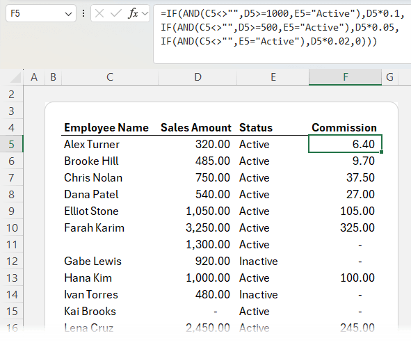
💡 The Fix: Use Helper Columns
Helper columns might sound “beginner,” but they’re an advanced design technique. They make your spreadsheets easier to audit, faster to calculate, and simpler to update.
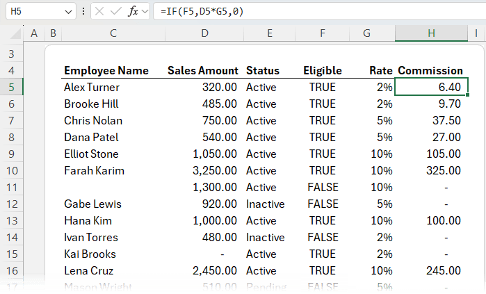
Example setup:
| Column | Formula | Purpose |
| Eligible | =AND(C5<>"", E5="Active") | Checks if employee has a name and is Active |
| Rate | =XLOOKUP(D5, CommRates[Sales Band], CommRates[Rate],, -1) | Finds correct commission rate |
| Commission | =IF(F5, D5*G5,0) | Multiplies sales by rate only if eligible |
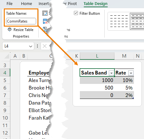
Now, if your commission bands change, just update your CommRates table. No formula rewrites required.
Rule 2: Boolean Logic – The Shortcut Pros Use Instead of IF
Remember that last formula?
=IF(F5, D5*G5, 0)
You can actually drop the IF entirely.
That’s because TRUE = 1 and FALSE = 0 in Excel.
So this works perfectly:
=D5*G5*F5
When F5 is TRUE (1), it multiplies as normal. When FALSE (0), the result is zero.
✅ Cleaner. ✅ Faster. ✅ Easier to read.
That’s the magic of Boolean logic. Excel’s hidden shortcut for smarter formulas.
Rule 3: Use Invisible Helper Columns with LET
If you love clarity but hate clutter, the LET function is your best friend. It lets you create variables inside your formula, turning long logic chains into readable sentences.
Example:
=LET(
eligible, AND(C5<>"",E5="Active"),
rate, XLOOKUP(D5, CommTbl[Sales Band], CommTbl[Rate],,-1),
D5*rate*eligible
)
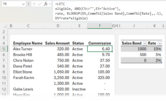
Here’s what’s happening:
- ‘eligible’ checks name and status
- ‘rate’ looks up the correct commission band
- The final calculation multiplies everything together
Result: the same output as before, but with no helper columns, and a formula that reads like a story.
👉 Want to master LET? Watch my full LET tutorial for syntax, debugging tips, and performance insights.
Rule 4: Make Formulas Reusable with LAMBDA
The LAMBDA function turns any formula into your own custom Excel function, no VBA required. It makes it easy for less experienced users to perform complex calculations with ease.
Start by copying your LET formula, then wrap it in LAMBDA and replace the cell references with the LAMBDA variables like this:
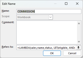
=LAMBDA(sales, name, status,
LET(
eligible, AND(name<>"", status="Active"),
rate, XLOOKUP(sales, CommTable[Sales Band], CommTable[Rate],, -1),
sales* rate * eligible
)
)
Go to the Formulas tab and save it in the Name Manager. I called it COMMISSION:
Now anyone can use it:
=COMMISSION(D5, C5, E5)
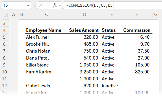
No long formulas. No logic errors. Just plug in the values and go.
This is modular Excel design. Formulas built once, used everywhere.
🧠 Want to go deeper? My Advanced Excel Formulas Course covers LET, LAMBDA, modular formula architecture, and more, step by step.

Rule 5: Think in Arrays, Not Rows
If you learned Excel before 2020, you probably think row by row.
But modern Excel works in arrays - one formula that spills down and across multiple cells automatically.
Example: Filter and Sort Active Employees
=SORT(
FILTER(C7:F29, E7:E29="Active"),
2,
-1
)
This shows all active employees, sorted by sales, in a single formula.
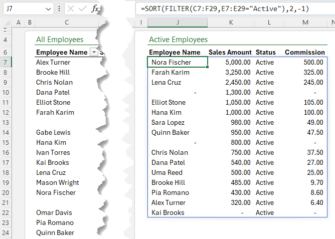
When data changes, it updates instantly. Add a new employee or change a status, Excel handles it.
Understanding the “Spill Range”
- The formula “spills” into adjacent cells automatically.
- You can’t type into the spill area (or you’ll get #SPILL! error).
- Reference the entire spilled array with a #, e.g. =J7#.
When Not to Use Arrays
Arrays are powerful, but not always ideal:
- When a simpler function (like SUMIF) will do
- When working with very large datasets (use Power Query or PivotTables)
- When formulas get too complex to debug
The Takeaway
These 5 hidden rules: helper columns, Boolean logic, LET, LAMBDA, and arrays are what separate “it works” spreadsheets from professional-grade models.
Each one helps you:
- Write faster formulas
- Debug with confidence
- Future-proof your workbooks

Folks who object to helper columns (or have bosses who do) can put all such things on a “helper page” that can even be hidden if desired. Then the helper columns they create will not affect the presentation aspect of their pages which some might value. Including many inheritors of age-old spreadsheets who cannot actually change layouts because “everyone’s used to them.”
One can even populate such a page with tables built using Power Query on the underlying data thereby gaining much capability in massaging the data that is put out to the sheet everyone thinks is the age-old sheet. So, mainly, not having to cobble together often somewhat arcane formulas that don’t really handle all the variations that arise in the underlying data. You know, because the data stream often DOES evolve even if the spreadsheet does not. PQ isn’t just for collection and some degree of massage. It can replace formulas thereby doing some or all of the manipulation of the cleaned data, with more range available, not to mention the automation.
But helper pages can at least overcome the “it’s STILL wholesale changes breaking lots of formulas that were never written for changes in the presentation scheme.
On the other hand, I’d point out that the helper columns added could be like the ones you added in that they can actually add comprehensibility to the presentation and not just the formulas in cell.
For instance, one might have a six factor formula but users who chronically wonder which factor or factors caused the result. Seeing a column of Yes/No or equivalents for, say, “eligibilty” might make such presentations much more acceptable to users since they’d no longer have to delve into the formulas to track down where a critical aspect occurred.
Not to mention that if they don’t need to keep diving into the formulas, then they don’t need to conserve the formulas to maintain their ability to understand them. Then one might have a far freer hand rebuilding to do things better, and even major presentation revamping. Which can lead to permission for something like a pivot table where such had always been denied before.
Thanks for sharing your experience and ideas, Roy. Very helpful.
Hi Mynda,
Thanks for another of your excellent tutorials. From having 38 of this formula -=IF(@$F$7:$F$2528=$F$2630,$H$2630, on a sheet, I now have =LET(
eligible, AND(F18″”),
rate, XLOOKUP(F18, Table5[Column1],Table5[Price],,),
eligible*rate), which is great if I need to adjust prices.
Awesome to hear, Tom! Might be a typo, but should there be a not equals sign in the AND formula, in fact, AND is redundant here as there’s only one criteria:
Hi Mynda,
To clarify: I adopted the formula –
eligible is the “permit type sold” in F18; no other criteria are required
Table5[Permits] (corrected) contains all permit types.
Table 5 [Price] returns the corresponding cost of the particular permit.
The spreadsheet is for our fishery, which includes all the types of fishing permits sold daily and their corresponding prices.
Regards, Tom.
“eligible is the “permit type sold” in F18; no other criteria are required”, ok, but this formula is just checking if the cell is empty or not. If you need to validate the type of permit, you might want to modify the formula to something like:
Replace “Valid Permit” with whatever your permit type is.
Mynda
Hi Mynda,
and thanks as ever for clear, informative and useful emails/pages. Any comments suggesting that information is missing is certainly what the Germans call, “Jammern auf hohem Niveau”, but given that three of the five functions, LET, LAMBDA and spillable arrays are only available on Office 365 and recent (2021, 2024, 2021) standalone Excel versions, a link to the Microsoft Excel function list with link text to the effect that users of standalone Excel versions could check the list to see whether functions mentioned are available on their installation may not be out of place. The list includes version markers to indicate the version of Excel a function was introduced. These functions aren’t available in earlier versions.
The list is also a useful general resource.
Great idea, Chris.