The INDIRECT function in Excel might seem like a clever solution, turning text into live references and helping build dynamic models but beneath the surface, it can wreak havoc on your workbook.
In this post, we’ll explore why INDIRECT causes more problems than it solves and walk through better, modern alternatives that are faster, more reliable, and easier to maintain.
Table of Contents
- Watch the Alternatives to INDIRECT Video
- Get the Excel Example File
- Why People Use INDIRECT
- The Problems with INDIRECT
- Better Alternatives to INDIRECT
- Want to Automate This?
- Use SWITCH Instead of Named Range Toggles
- Use FILTER and XLOOKUP for Dependent Drop-down Lists
- Final Thoughts: Move On from INDIRECT
- Next Step: LAMBDA
Watch the Alternatives to INDIRECT Video

Get the Excel Example File
Enter your email address below to download the free file.

Why People Use INDIRECT
Let’s start with the basics.
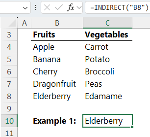
INDIRECT takes a reference in text form and turns it into a usable Excel reference.
For example, in the screenshot below, in cell C10 you can see =INDIRECT(“B8”) returns the value in cell B8, ‘Elderberry’:
INDIRECT also works with:
- Cell references: =INDIRECT("Sheet1!B8")
- Named ranges: =INDIRECT("Q1Sales")
- Combined references using concatenation: =INDIRECT("B" & C13)
This gives you the power to construct references on the fly, switch between named ranges, or dynamically pull values from various sheets.
It feels advanced, and it was, back in the day.
The Problems with INDIRECT
Despite its flexibility, INDIRECT has major downsides:
❌ Volatile: INDIRECT recalculates every time anything changes in your workbook, even if the change doesn’t affect the formula. This slows things down.
❌ Breaks easily: Rename a worksheet or a range? INDIRECT won’t update, it just breaks.
❌ No external links: INDIRECT can’t reference closed workbooks.
❌ Hard to debug: Since INDIRECT builds references invisibly, tracing errors becomes tricky.
Bottom line: it makes your workbook fragile.
Better Alternatives to INDIRECT
Let’s look at smarter, more modern options for common INDIRECT use cases.
✅ Use Power Query to Combine Data from Multiple Sheets
Instead of:
=XLOOKUP(A2, INDIRECT("'" & B2 & "'!A2:A10"), ...)
Try this:
Use Power Query to load all tables dynamically, even if they’re on separate sheets or different workbooks.
Steps (see video for step-by-step instructions):
- Format each sheet’s data as a table (e.g., FY2025_01, FY2025_02, etc.)
- In Power Query, use =Excel.CurrentWorkbook() to list all tables
- Filter to include only the ones you want (e.g., names starting with FY)
- Expand and combine them into one table
- Clean and reshape the data
- Load to a PivotTable
✅ One refresh updates everything
✅ No fragile formulas
✅ No performance issues
Want to Automate This?
If you’re ready to take your Excel skills up a notch, check out our Power Query course. You’ll learn how to:
- Merge and clean messy data
- Automate repetitive tasks
- Build reports that update with a click
Thousands have used it to ditch unreliable formulas and save hours each week.
Use SWITCH Instead of Named Range Toggles
If you're toggling between named ranges like Q1Sales and Q2Sales, ditch INDIRECT:
Instead of:
=SUM(INDIRECT(G5))
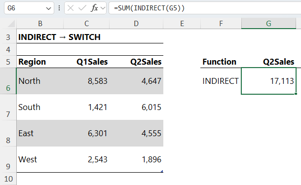
Use:
=SUM(SWITCH(G5,
"Q1Sales", TblSales[Q1Sales],
"Q2Sales", TblSales[Q2Sales]))
✅ No need to define extra names
✅ Easy to audit
✅ Much faster to calculate
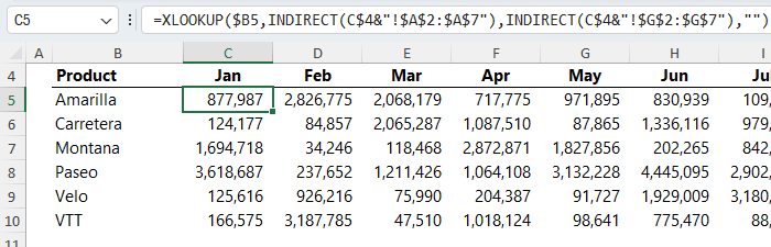
Use FILTER and XLOOKUP for Dependent Drop-down Lists
Many people use INDIRECT to create dependent drop-downs, where the second list changes based on the first.
Instead of INDIRECT, use FILTER:
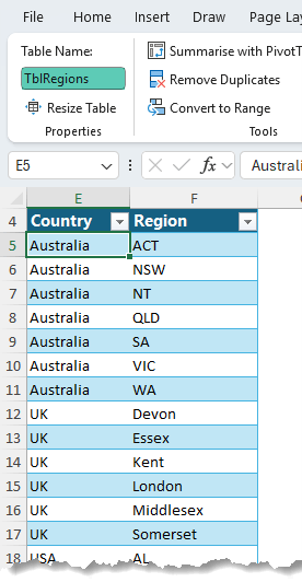
1. Structure your data as a two-column table: e.g., Country | Region
2. Format it as a table (mine is called TblRegions)
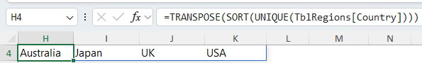
3. Use this formula to extract a list of countries sorted A-Z:
=TRANSPOSE(SORT(UNIQUE(TblRegions[Country])))
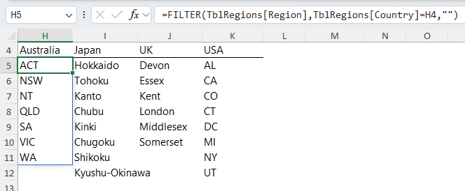
4. Use this for regions based on the selected country in H4:
=FILTER(TblRegions[Region], TblRegions[Country]=H4, "")
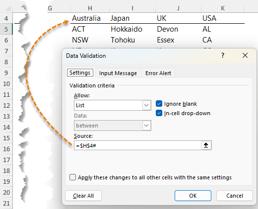
5. For dynamic data validation go to the Data tab > Data Validation > List:
- For the Countries drop down list use this formula in the Source:
=$H$4#
- Regions:
=XLOOKUP(B5, $H$4:$P$4, $H$5:$P$5)#
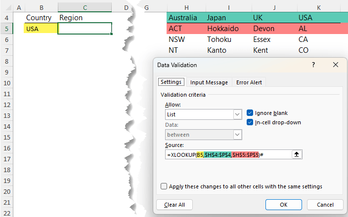
Tip: the hash sign on the end of the XLOOKUP formula tells Excel to return all the results in the spilled array in row 5, not just the first result.
This approach to dependent drop-down lists is:
✅ Fully dynamic
✅ Works in Excel 365, 2021, and Excel Online
✅ No volatility
Final Thoughts: Move On from INDIRECT
If you’ve been relying on INDIRECT to build flexible models, it’s time to modernize. Excel now offers:
- Power Query for data transformation
- FILTER and XLOOKUP for dynamic logic
- SWITCH for simple toggles
- LAMBDA for creating reusable custom functions
These tools are easier to manage, less error-prone, and won’t slow down your file.
Next Step: LAMBDA
If INDIRECT felt like a cool trick, LAMBDA will blow your mind. It lets you define your own Excel functions from formulas. Check out this comprehensive LAMBDA function tutorial to get up to speed.


I have two spreadsheets that calculate KPIs, called Booked Capacity and Diary Volume. Each of these have a few calculation tabs, and then the results are calculated on a separate tab per employee.
I now want to create a “Dashboard” spreadsheet per employee that the employee and their supervisor can access (read only). I’ve created the first few, but each is identical except for the name of the employee. To modify these, all I need to update is the tab name in the formulas. Is there a way to do this without using “indirect”?
Example formula to bring across data: =’…[Diary volume 2025.xlsx]Melissa’!$B$54:$AN$80
“Melissa” is all that needs to be updated per employee.
Hi Viv,
One way is to not create a separate tab per employee in the first place and instead create one dashboard that can be filtered using Slicers for the employee you want to view (I’m assuming this would be ok seeing you have all employee’s data in the one file already anyway).
Alternatively, use Power Query to gather the data from all the sheets into one table (in a tabular layout), then you can use PivotTables with Slicers to filter the dashboard to show the relevant employee, similar to the first option.
I hope that points you in the right direction. If you get stuck, please post your question on our Excel forum where you can also upload a sample file and we can help you further.
Mynda