Still typing out employee schedules by hand or dragging cells like it’s 2005? Let’s fix that with an automated work schedule in Excel.
This guide will walk you through how to build a dynamic, colour-coded employee schedule that:
- Automatically generates the dates for any month
- Calculates finish times from standard hours and start times
- Highlights days off, holidays, and sick days with drop-downs and colours
- Summarizes days worked, sick, and on holiday
- Looks good and saves hours each month
Of course, you can customize it to suit your unique requirements once you have the foundation.
Table of Contents
- Watch the Automated Work Schedule Video
- Get the Free Work Schedule Template
- Build a Smarter Work Schedule in Excel
- Step 1: Generate the Dates for the Month
- Step 2: Set Up the Employee Table
- Step 3: Add Drop-Downs for Work Status
- Step 4: Colour-Code Work Statuses
- Step 5: Automatically Calculate Finish Times
- Step 6: Freeze Panes for Easy Scrolling
- Step 7: Add Visual Dividers Between Employees
- Step 8: Create a Dynamic Heading
- Step 9: Add Summary Figures (Optional but Useful)
- Step 10: Customize and Expand
- Next Steps
Automated Work Schedule Video

Get the Practice File
Enter your email address below to download the free files.

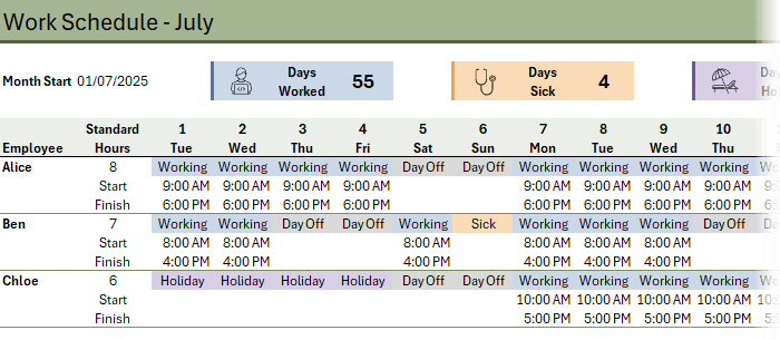
Build a Smarter Work Schedule in Excel (That Updates Automatically)
Watch the video above for step-by-step instructions on how to build an automated work schedule, or follow the written instructions below.
Step 1: Generate the Dates for the Month
1. In cell B3, enter the start of the month (e.g., 1/7/2025 for 1st July).
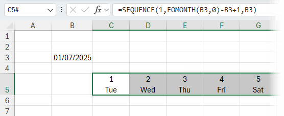
2. In C5, enter the following formula to spill the dates across the row:
=SEQUENCE(1,EOMONTH(B3,0)-B3+1,B3)
3. Format the date cells:
- Select the cells, press CTRL + 1 to open the Format Cells dialog.
- Go to the Number tab → Custom.
- Enter this custom format:
d CTRL+J ddd
(Press CTRL+J between the d and ddd to wrap the day name on a new line.) - Then, go to the Alignment tab:
- Check Wrap Text
- Set Horizontal Alignment to Center
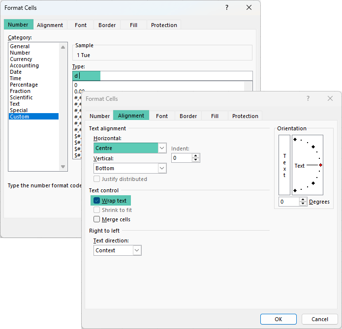
- Increase row height to fit the text.
It should look like this:
Step 2: Set Up the Employee Table
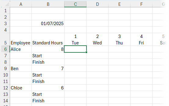
1. In column A, list your employees:
Example:
- A6: Alice
- A9: Ben
- A12: Chloe
Each employee needs 3 rows:
- Row 1: Work status
- Row 2: Start time
- Row 3: Finish time
2. In column B, input each employee’s standard work hours:
- B6: 8 (Alice)
- B9: 7 (Ben)
- B12: 6 (Chloe)
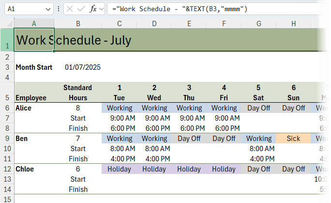
It should look something like this:
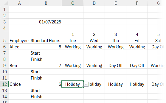
Step 3: Add Drop-Downs for Work Status
1. Select the first row for each employee’s schedule (e.g., C6:AG6 for Alice).
2. Go to Data > Data Validation > List and enter:
Working,Day Off,Sick,Holiday
(Add/remove options from the list to suit your requirements.)
3. Copy the data validation to each employee’s status row.
4. Set the work status for each employee for the month.
Mine looks like this now:
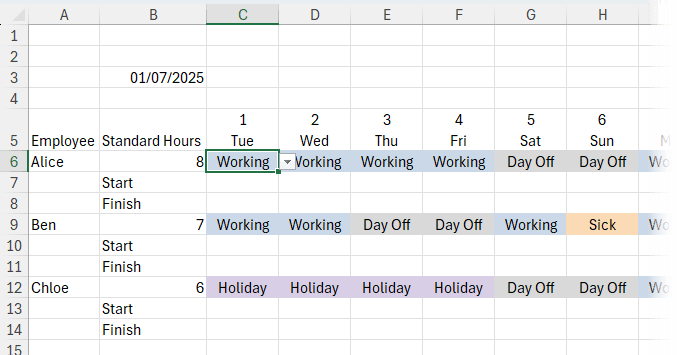
Step 4: Colour-Code Work Statuses
1. Select all status cells (e.g., C6:AG28 to allow space for more employees).
2. Go to Home > Conditional Formatting > Highlight Cells Rules > Text that Contains.
3. Add rules like:
- “Working” → blue fill
- “Day Off” → grey fill
- “Sick” → orange fill
- “Holiday” → green fill
It’s coming along nicely:
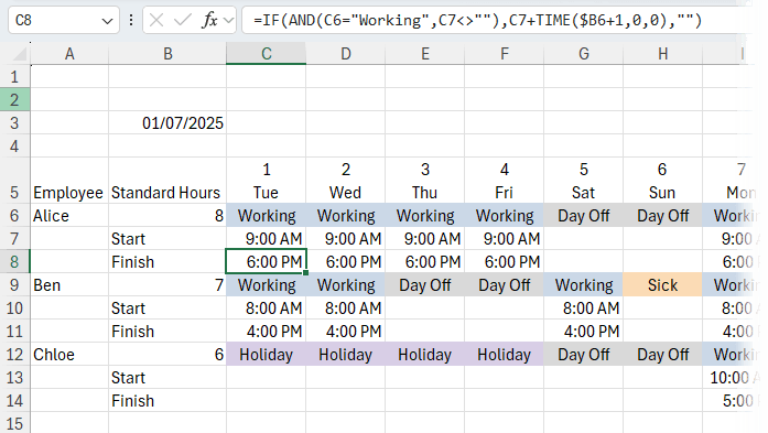
Step 5: Automatically Calculate Finish Times
1. In the second row for each employee, enter their start time (e.g., C7: 9:00 AM).
2. In the third row (e.g., C8), enter the formula:
=IF(AND(C6="Working",C7<>""), C7+TIME($B6+1,0,0), "")
This checks if the employee is working and has a start time, then adds standard hours +1 hour for lunch. Modify the +1 to suit your break duration.
3. Copy this formula across the row and down for other employees.
Step 6: Freeze Panes for Easy Scrolling
Select cell C6 > go to View > Freeze Panes > Freeze Panes
Now, names, standard hours and dates in row 5 stay visible while scrolling.ces (like Allocation), you can even skip the extra brackets after the @ sign:
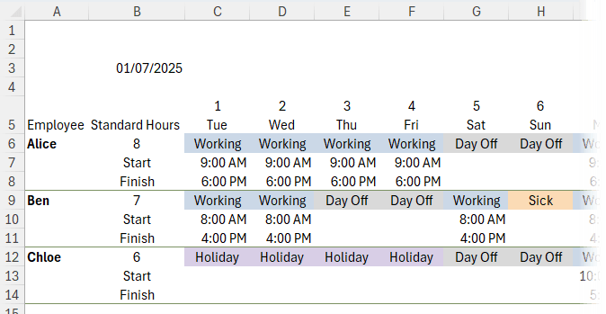
Step 7: Add Visual Dividers Between Employees
1. Select all rows in the schedule (e.g., A6:AG28)
2. Go to Home > Conditional Formatting > New Rule > Use a formula
Use this formula:
=$B6="Finish"
3. Format with a green bottom border to separate each employee’s block.
4. Go to the View tab and turn off gridlines.
Step 8: Create a Dynamic Heading
1. In cell A1, enter:
="Work Schedule - " & TEXT(B3,"mmmm")
2. Format this row with green fill and white bold text for visibility.
3. While we’re formatting, let’s also add green fill to row 5 and format the font bold.
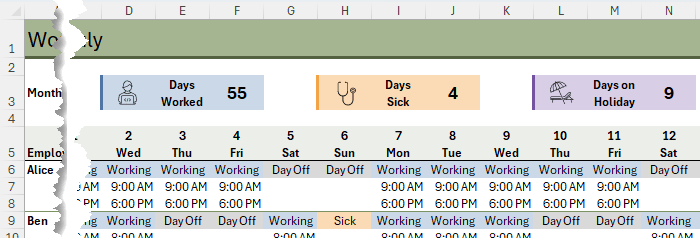
Step 9: Add Summary Figures (Optional but Useful)
1. Use COUNTIF to calculate how many days were worked:
- In E3: label = Days Worked
- In F3:
=COUNTIF(C6:AG30,"Working")
Repeat for “Sick” and “Holiday” if you want more summaries.
2. Add icons using Insert > Icons, search for:
- Computer (working)
- Doctor (sick)
- Sun (holiday)
Resize and colour to match your theme.
Step 10: Customize and Expand
You can change the standard hours, start times, or status drop-downs to suit your team.
To add new employees, just insert a new 3-row block and copy formatting and formulas.
Next Steps
If you enjoy this kind of logic-based setup and want to feel more confident using formulas like these, I teach everything from Excel formulas to dashboards and Power Query in my online Excel courses here.
These are the exact tools I rely on when building templates like this, and they’ll help you go from basic spreadsheets to time-saving systems.


the first formula the system give me a error that the formula has an error
=SEQUENCE(1,EOMONTH(B3,0)-B3+1,B3)
It may be that you don’t have the SEQUENCE function in your version of Excel. If you type =SEQ does SEQUENCE display in the auto-complete? If not, that’ll be the reason.
How do I MAKE THIS FORMULA CALCUALTE THE HOURS BIWEEKLY so that we could see if they worked 80 hours AND THEN ALSO DO MILITARY TIME INSTEAD OF 12 HOURS TIME
Please post your question on our Excel forum where you can also upload a sample file and we can help you further.
Hi, I would like to know which MS Office Version is this lesson workable?
Hi Lillien,
This works in Excel for Microsoft 365 or Excel 2021 onwards. If you have an earlier version of Excel, you can generate the dates manually or using a slightly different formula. If you get stuck, please post your question on our Excel forum where you can also upload a sample file and we can help you further.
Mynda
Schedule for the employee monthly shift change calendar duration after 21 days…. night to day and day to night……tq
Feel free to modify the schedule to suit your needs, Prakash. If you get stuck, please post your question on our Excel forum where you can also upload a sample file and we can help you further.