Excel Tables are brilliant for structured data and dynamic formulas, but if you’ve ever copied a formula across columns and ended up with unexpected results, you’re not alone. The issue? Table references behave differently depending on how you copy them - and Excel doesn’t give you a straightforward way to lock them like with normal cell references.
In this guide, you’ll learn how to lock table references the right way - plus a smart shortcut to save time.
Table of Contents
- Excel Table Absolute Structured References Video
- Get the Practice File & Cheat Sheet
- The Problem with Copying Excel Table Formulas
- Locking a Single Column Reference in a Table
- Shortcut to Insert Table Structured References Quickly
- Locking Multiple Columns in Table References
- Making Multi-Column References Relative
- Locking Row References in Excel Tables
- Referencing Rows in a Table
- Cheat Sheet: Table Reference Syntax
- Final Thoughts
Excel Table Absolute Structured References Video

Get the Practice File and Cheat Sheet
Enter your email address below to download the free files.

The Problem with Copying Excel Table Formulas
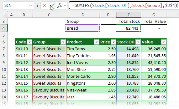
Let’s say you’re using a formula like this:
=SUMIFS(Stock[Stock OH], Stock[Group], $D$4)
This sums the “Stock OH” column based on a “Group” match in D4 as shown below:
Sounds great… until you copy it.
- Copy/paste (Ctrl+C, Ctrl+V): Structured references are treated as absolute. That means they don’t shift when pasted - great if that’s what you want, but usually it’s not.
- Left-click and drag: Structured references are treated as relative. When you drag the formula across, the column references shift - and your formula breaks:
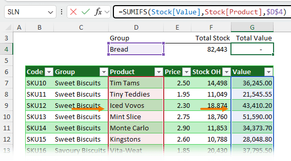
So, how do you lock a specific table reference?
Locking a Single Column Reference in a Table
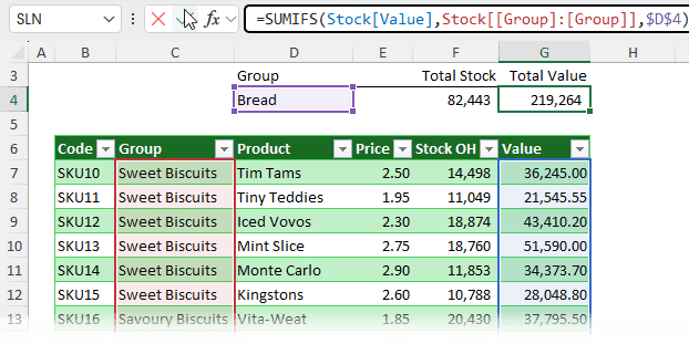
To lock a column like Stock[Group], wrap it in an extra set of square brackets and repeat the column reference like this:
Stock[ [Group] : [Group] ]
Note: Spaces added for clarity.
This tells Excel: lock the reference from the Group column to the Group column - essentially, just this column.
Now when you drag the formula across, it won’t shift.
Shortcut to Insert Table Structured References Quickly
Instead of manually typing double brackets and colons, select two columns in the formula editor. For example:
Stock[[Group]:[Product]]
as shown below:
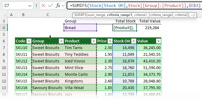
Then just replace ‘Product’ with ‘Group’ and you're done. Excel writes the double brackets and colon etc. for you, plus no memorizing syntax required.
Locking Multiple Columns in Table References
Double brackets work for ranges too:
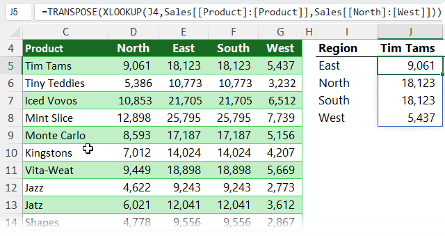
=XLOOKUP(J4, Sales[[Product]:[Product]], Sales[[East]:[West]])
- The first part looks for a match in the Product column (locked).
- The second part returns values from East to West (locked by default when multiple columns are selected with your mouse).
To return these horizontally but spill vertically, wrap it in TRANSPOSE (see screenshot below):
=TRANSPOSE(XLOOKUP(J4, Sales[[Product]:[Product]], Sales[[East]:[West]]))
Making Multi-Column References Relative
By default, Excel locks multi-column references like:
=SUM(Sales[[North]:[East]])
Copy it across and it won’t shift.
To make it relative, remove the double brackets and prefix each column with the table name.
=SUM(Sales[North]:Sales[East])
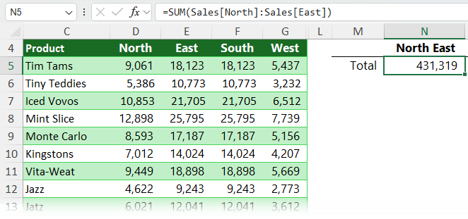
Now it will shift when copied across - perfect for side-by-side calculations.
Locking Row References in Excel Tables
When working inside a table, Excel uses the @ symbol to refer to values in the current row:
= [@Allocation] * [@[Admin Overhead]]
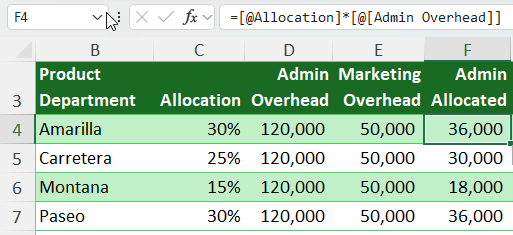
Drag it across and - uh oh - it shifts columns.
To lock it:
1. Select a multicell range across columns like cells C4:D4, Excel will insert the structured reference with the double brackets and colon already inserted:
=Overheads[@[Allocation]:[Admin Overhead]]
2. Then replace the second column with the actual one you want and complete your formula:
= Overheads[@[Allocation]:[Allocation]] * [@[Admin Overhead]]
Now it's locked.
Referencing Rows in a Table
You can also reference multiple columns in the same row:
=SUM(Overheads[@[Admin Allocated]:[Marketing Allocated]])
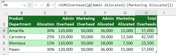
This sums across columns in the same row.
Tip: If the column name has no spaces (like Allocation), you can even skip the extra brackets after the @ sign:
=[@Allocation]
Cheat Sheet: Table Reference Syntax
I know there’s a lot of scenarios, so I included this cheat sheet in the Excel file you can download above to help you quickly find what you need:
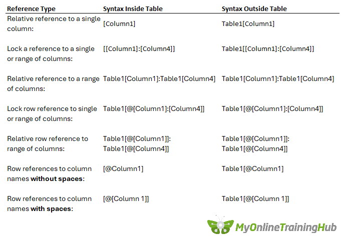
Tip: Don’t try to memorize these - just use the mouse and have Excel insert them for you, then tweak as needed.
Final Thoughts
Locking structured references isn’t always intuitive, but once you know the double bracket trick and the mouse shortcut to insert them, it becomes second nature. Whether you’re locking rows, columns, or ranges, the key is using the right syntax for the right copy method.
Are you using Excel Tables to their full potential? See what else Tables can do, check out our comprehensive Excel Tables lesson here.


Eye roll at people who love structured references.
Show us how to do a fairly simple accumulation sumif based on multiple columns.
If I see that done, maybe then I’ll start giving them some love.
I agree, referencing multiple columns isn’t the most intuitive, but like anything, once you get the hang of it it’s not that difficult. That said, don’t forget you can submit ideas for improvements to Excel on UserVoice.
Excellent. You are the best of all I have seen ! Thank you very much
Thank you! Glad you found it helpful 🙂
Really wonderful excel data informations. Even only 20 pages but for me are really
more than that. Thank you very much !!
Glad you found it useful, Shaoyuan 🙂
Great article. I use Absolute structured references all of the time, but I still learned something.
I have a reoccuring issue… I export excel data from my eCommerce components. These components are in active development, and from time to time the structure of the excel export will change, e.g. new columns added or simply ordering changed.
For example, previously, my excel export had the following column order…
Date Submitted, club, clubid, feedback, comment, email, ChildsName.
I pasted this into my “Data” table
I had another table which analysed the raw data, and the following formula counted the number of people who gave feedback of 3 (column in Analysis table has heading = “3”…
=COUNTIFS(Data[[feedback]:[feedback]],Analysis[[#Headers],[3]],Data[[clubid]:[clubid]],Analysis[[ClubID]:[ClubID]])
After a recent excel update, the excel export has a different order
Date Submitted, club, feedback, comment, email, ChildsName, clubid
When I paste this into my “Data” table, the formulas in my Analysis table get changed to…
=COUNTIFS(Data[[comment]:[comment]],Analysis[[#Headers],[3]],Data[[feedback]:[feedback]],Analysis[[ClubID]:[ClubID]])
This is incredibly infuriating, as my reports keep breaking, as the developers work their magic on the eCommerce components. Is there a way to write my analysis formula, so that absolute structured references will always refer to the correct column, while remaining absolute?
Thanks for any help you can provide.
There are a few ways out of this situation. Are you using excel 2010 or higher? You can try Power Query in this case, to import the new data into your Data sheet.
Another way out is to use vba to import data by columns, this way your Data headers will always remain the same, and you will import the corresponding columns from the source file into the correct column.
Changing data headers in the destination file, to match the position of the source columns, will allow you to paste only data, not headers. By default, when you rename a column in a table, excel will automatically update that name in all formulas from that workbook, and this is a very good behavior, but in your case, pasting data including headers is not a good option. Rearranging columns in a defined table is easy, just drag the header cell in the position you want.
Catalin
Is there a way to refer to a cell in a seperate table using lookup criteria from the initial table? I got errors with power pivot since my data contains too many duplicates to create relationships. Essentially I want to compare Bob’s budget each month to his forecast in a seperate table, while avoid using a vlookup to ease reading the formula. If combinations of syntax or structured references can look up say an employee number in a range of rows of the other data table, that would be great
Hi Alexander,
That’s what Power Pivot does. Load your lookup table to power pivot and add a relationship between data table and lookup table, that’s all you need.
Or, you can load to data model both the data table and the lookup table, and you can merge them into a single table.
Catalin
Mynda,
This is great. There is always so much to learn with Excel. Favorite part by far is how to actually use absolute referencing structured references.
Honestly because of the flexibility of Excel Tables to expand without having to use offset formulas in name ranges, why wouldn’t you want to use them all of the time.
Thanks
Brad
I agree completely, Brad 🙂 I’m happy to put up with the few limitations of Tables to have the structured reference functionality.
Mynda
Dear Phil & Mynda,
Thanks for an excellent tutorial and a superb add-in. I will personally thank Jon on his website.
You have a knack of coming out with something new / arcane everytime you post. So glad to receive your tips.
Thank you very much!!!
Adi 🙂
Thanks, Adi 🙂 That’s wonderful to know.
Mynda
Very good tip. Easier option. Thanks for sharing.
Thanks Jef.
Awesome trick. Thank you very much.
Thanks, Rajesh 🙂
Hi Mynda
Another good tutorial from you about some tricky Excel functionality. However, whilst structured referencing has some advantages, I find them a pain in the proverbial :-(, because:
(1) the “ease of deciphering” the formula is outweighed by the time-consuming fiddling around that is required to make the references absolute or relative as required, and
(2) what appears to be the inability to have relative referencing when copying and pasting a structured reference. Copying and pasting of formulae and utilising the absolute/relative referencing that comes with that is one of the absolute fundamentals (pardon the pun) in the use of Excel. One should not have to drag across columns / down rows (or use fill handle?) to have structured references remain relative! What if your table has hundreds or thousands of rows/columns – dragging or using the fill handle should NOT be the only option.
If I’ve missed something about using structured referencing with Excel tables that overcomes the latter problem when copying, I’d be very happy to be enlightened.
Regards
Col
Hi Col,
I agree that they are fiddly and should be more user friendly, although Jon’s free addin goes a long way to fixing their limitations.
While the fill handle requirement is a pain I find if I drag it across the columns where required, I can then double click the bottom right corner of the cell containing my new formula to fill it down the column, so it’s a bit more painful than a regular formula but still worth the while.
For me the benefits of the dynamic ranges that are built into Excel Tables makes them worth using and putting up with their absolute reference hassles.
I hope that the absolute/relative limitations might be fixed in a future Excel release, however I don’t have any inside info on that, it’s just my wish!
Mynda
Is there a downloadable Excel Workbook to follow along?
Hi Babak,
I’ve added a link to the post (towards the top) where you can download the workbook 🙂
Mynda
Thank you Mynda! This is a great tutorial. I did not know about the relative references to multiple columns. That’s a great trick that I will have to incorporate into the add-in.
Have a good one! 🙂
Cheers, Jon 🙂
I hope everyone loves your add-in as much as I do.