In Excel there are two almost identical functions; SEARCH and FIND.
The SEARCH and FIND functions allow you to find the location of text within a string of text.
They’re identical because they perform the same function except the FIND function is case sensitive, whereas the SEARCH function is not, and SEARCH allows the use of wildcards whereas FIND does not.
So let’s look at how we can use them.
SEARCH Function
The syntax for the SEARCH function is:
=SEARCH(find_text, witin_text, [start_num])
In English:
=SEARCH(find the location of my text or my text string, within a cell containing text or a text string, starting from position x)
Note: if the [start_num] is omitted it will start at 1.
For example; if cell A1 contains the words ‘went away’ and your formula reads
=SEARCH('E',A1)
The result will be 2, since the letter ‘e’ is the second letter in cell A1.
If you wanted to search for a text string, let's say ‘away’
=SEARCH('away',A1)
The formula would return the result 6, since the word ‘away’ starts in position 6 in cell A1.
SEARCH Function Examples
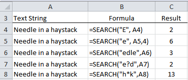
SEARCH Function Examples Explained:
- You’ll notice in the first example the SEARCH function ignored the fact that we were searching for an upper case ‘E’ and still returned a 2. If you want case sensitivity use the FIND function.
- In the second example we put the start_num as ‘4’ and the result was 6.
- In the third example we wanted it to return the starting position of a text string ‘edle’ so Excel ignored the first ‘e’ and returned the result ‘3’.
- In the fourth example we used a question mark wildcard. The question mark wildcard will return the position of text that begins with an ‘e’, then has any single character, and ends in a ‘d’.
- In the fifth example we used an asterisk wildcard. The asterisk wildcard enables us to search for any string that begins with an ‘h’ and ends in a ‘k’.
- If the text string is not found the SEARCH function will return a #N/A result.
Note: you can’t use wildcards with the FIND function.
Whoop-de-doo I hear you say. What will I ever use that for? Ok, I hear you.
Some Cool Uses for SEARCH and FIND
On their own SEARCH and FIND aren’t much use so let's look at some ways to use them nested in other formulas to unleash their power!
Enter your email address below to download the sample workbook.
- Convert the result to a TRUE/FALSE answer using ISNUMBER and then use it in an IF statement to return a value for 'brown foxes' and a different value for everything else.
- Use with MID to parse columns as an alternative to Text to Columns
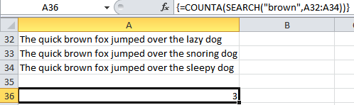
- Use it as an array formula to count the number of instances of a word occurring in text strings in a range of cells.
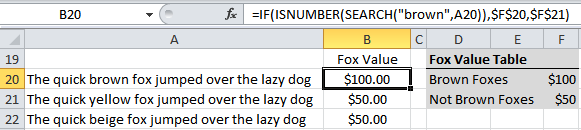
Brief Explanation: The formula in cell B20 is searching for the word ‘brown’, if the result is a number (ISNUMBER) then choose the value in cell F20, and if it’s not (if the word isn’t found SEARCH will return a #N/A error) then choose the value in cell F21.
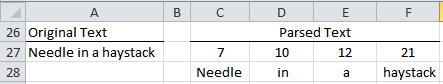
In cell C27:
=SEARCH(" ",A27)
returns the position of the first space, which is also the length of the first word (including the space).
In cell
D27:
=IFERROR(SEARCH(" ",$A$27,C27+1),LEN($A$27)+1)
Finds the location of the second space.
If the result is an error it returns the length of the whole text string + 1. This is simply error handling as the last word in the text string will return a #VALUE! error without this.
In cell C28:
=MID($A$27,1,C27)
returns the first seven characters in the cell A27.
In cell D28:
=MID($A$27,C27,IFERROR(D27-C27,100))
Again, the IFERROR is simply error handling for the last word in the text string.
Now you can copy the formulas in D27 and D28 across your columns as many times as required, and Bob’s your Uncle!
Brief Explanation: This example uses the SEARCH function to locate the starting position of each word in cell A27.
It does this by finding the location of each space, and then adding 1 to get the starting position of each word.
It then uses those numbers in MID formulas in row 28 to extract the individual words from cell A27, and puts them in their own column. Just as you can do with Text to Columns.
This requires 4 different formulas, but once you’ve set them up you can copy them across your columns and quickly parse large amounts of text.
Note: the formula is entered
=COUNT(IF(SEARCH("brown",A32:A35),1,""))
and then you press CTRL+SHIFT+ENTER to enter it as an array formula and Excel will enter the curly brackets for you.
If you liked this let me know by clicking the Facebook like, Tweet it or simply leave a comment below. I'd love to hear from you and how you use these functions.
Searching for Text Strings in Power Query
We can also use Power Query to search for text strings, including case and non-case sensitive searches.

great solution to correct existing spreadsheets where someone but multiple data elements in a single cell, without a lot of manual labor!
Alright. I’m going to try to explain my question in words as best as I could…
Is there a way… to use the search and isnumber functions together with a vlookup or sumif or similar function? I have a table (I’ll call it “tracking”) with months across the top (Jan15, Feb15 etc.) and Vendors listed down the side, which I need to populate with either a YES or NO depending on whether we received payment on them for the given month. I have the data spreadsheet set up so that if a vendor pays one check for months Jan-Mar you could type into the Month Paid column, “jan14,feb14,mar14” to show that they paid those months. This could then be searched using the column headers on my tracking table and together with the isnumber function, it’ll yield a “YES” if there’s a number or “NO” if not. My issue is that as vendors send in checks, they’re recording in the next available row on the spreadsheet. How can I use this search function to search the Month Paid column only if the vendors match? Also, I would need it to search through the entire column for all occurrences of that vendor to see if in any of those rows, searching the Month Paid column would result in a value for our respective month column.
I apologize if this is really confusing.
Thanks,
David
HI David,
Please upload a sample file with your data structure, to see how data is organized. You can use our Help Desk, it will be easier to understand the problem. Any detail you can give is important, so be generous with details 🙂
Cheers,
Catalin
I have a list of 7000+ words and want to search it with variables such as, find all words where the third character is “u”, or where the third character is “u” and the fifth character is “d”, for example. Not sure how to do this? Many thanks.
Hi Alf,
Use a filter to find those values. Assuming that your list starts from A1, and it has a header cell, select A1, from ribbon choose Data and press the Filter button; in cell A1, you should have a dropdown button, a column filter; from that menu, choose Text Filters–> Begins With, and type this : ??u to see only the words that have a “u” as the third char, or type ??u?d to filter only the words that have third char u and fifth char “d”. The question mark represents a single unknown character.
Cheers,
Catalin
Great; thanks!
You’re wellcome 🙂
My excel file name is not “generation_mart.xls” I want insert file name in work sheet but only the part generation. can you help
Hi Kevin,
The following formula:
=LEFT(MID(CELL("filename",F9),FIND("[",CELL("filename",F9))+1,LEN(CELL("filename",F9))-FIND("[",CELL("filename",F9))),FIND(".xl",MID(CELL("filename",F9),FIND("[",CELL("filename",F9))+1,LEN(CELL("filename",F9))-FIND("[",CELL("filename",F9))))-1)will return the entire name of the workbook. If you want to return a partial name, replace:
FIND(".xl" with FIND("_"This will return the all characters until
is found.
Catalin
I’m get error, it highlight the (“[“
Try retyping the double quotes from keyboard, it might be a problem when copying formula from web page. (the web page replaced the quotes with other characters)
Catalin
I have a list of twenty words in one column and want search for that list in another column and where every one of twenty words is found, the word itself should be place beside the cell of the other column.
Hi Kevin,
This is usually done with VBA programming, it’s too complicated to do it with built in functions.
Upload a sample workbook on Help Desk, maybe we can find a solution for you.
Catalin
This is lovely it has realy helped me alot. pls i have a data that have Date, Time and Values in A1,B1 and C1 respectivelly. The Date is down to A20 with the Time and Values as well.I used (=max(C2:C20) to get the maximum value, how can i search or look for the Date or Time at which the max value occur
Hi Joseph,
You can find the row number of the max value with:
=MATCH(MAX(C1:C20),C1:C20,0)
This result can be used in the second argument of the INDEX function, to return the corresponding values from column A or B
The first sentence of your article solved my problem. Thanks!
Wow, that was easy! Thanks, Narayana 🙂
Hi Ms Mynda
I’ve one question :
I want find a “◘” in the cell and anywhere that find “◘”, All cells get sum and show the result in a cell
Hi Mahyar,
You need to use the CHAR function to translate the symbol into a character code that Excel can recognise. Your formula might be:
You can find out what the character code is by finding it in the Insert Symbol dialog box. At the bottom of the dialog box is the Character Code. You need the ASCII version.
Kind regards,
Mynda.
Hi Ms Mynda.
Thanks for your guidance. I thought and found it solution.
My answer was:
=SUMIF(F7:F15;”◘”;D7:D15)
I’ll test your formula, I think,I need .
Good Luck
Hi Mynda,
Can you spread some light on the below issue.
In A1 i have mink12? and the formula in B1 is
=SUMPRODUCT(SEARCH(MID(A2,ROW(INDIRECT("1:"&LEN(A2))),1),"0123456789abcdefghijklmnopqrstuvwxyz!@#$%^&*()_{}][ "))Result is 72 instead of error because question Mark(?) is not there in the search list i mentioned in the formula.
Similar issue is with ~ as well.
Thanks
Minku
Hi Minku,
The asterisk, question mark and tilde are wildcards in Excel and will be affecting your formula. You can read more on wildcards here.
Kind regards,
Mynda.
Hi Mynda,
I gone through the link you provided and tried but it is not working.
Can you suggest idea to perform this task.
Thanks
Minku
Hi Minku,
I get 93 not 72. It counts the ? as a 1 even without it in the character list.
If you use the Evaluate Formula tool on the Formulas tab of the ribbon you can step through the formula as it evaluates to see what it’s doing.
If 93 isn’t what you want can you please let me know what outcome you’re expecting and why.
Thanks,
Mynda.
Hi Mynda,
I still get outcome 72 instead 93.
Items mentioned in the formula are the permitted characters. Formula is to check whether string in the cell contain any characters which is not mentioned in the list.
min?123
So as per the formula question mark is not in the list hence it should give ERROR like #Value else if all the characters from the string are there in the list then the outcome of the formula should be numeric value.
Let say if question mark is not there in the list, then according to the below formula outcome should error.
=SUMPRODUCT(SEARCH(MID(A2,ROW(INDIRECT(“1:”&LEN(A2))),1),”0123456789abcdefghijklmnopqrstuvwxyz?!@#$%^&*()_{}][ “))
Regards
Minku
Hi Minku,
I understand now. There seems to be a problem with SEARCH evaluating the ? to position 1 in the text string.
This formula evaluates correctly:
=SUMPRODUCT(FIND(MID(A2,ROW(1:100),1),"0123456789abcdefghijklmnopqrstuvwxyz!@#$%^&*()_{}][ "))Note: FIND is case sensitive so you will need to add capitals to your text string if your data contains capitals too.
Thanks to Roberto for helping me with this solution.
Kind regards,
Mynda.
Hello
I am facing a problem in writing formula.
Objective is to search whether item or items in the list present in the string or not.
List contains name of continents, lets say F1 to F7.
String in A1 Indiaasia
A2 canadanorth America
A3 AfricaIndiaEurope
Is there any way i can right formula for the same.
Thanks
Hi Minku,
You can wrap the SEARCH function in ISNUMBER to return a TRUE or FALSE outcome. Like this:
=ISNUMBER(SEARCH("asia",$A$1:$A$3))=TRUE
Kind regards,
Mynda.
Hi Mynda,
Thanks for the quick reply, but i am still facing problem with formula. Search formula giving me one to one search.
For example in my spread sheet F1 to F7 continent names & in the following order.
Asia, Africa, North America, South America, Europe, Antartica and Australia.
In cell C1 to C3 i have Indiaasia, KenyaAsia, canada Europe.
When i enter formula in E1 as {Search($F$1:$F$7,C1)} it gives me Asia but when i enter same formula in C2 it gives error.
Hi Minku,
I see the whole picture now….I think 🙂
If you want to check if the values in column F are present in column C you can use this formula:
=ISNUMBER(MATCH("*"&F1&"*",$C$1:$C$4,0))It will give you a TRUE or FALSE outcome. i.e. it will give you a TRUE for Asia and Europe and FALSE for the others.
Kind regards,
Mynda.
I’m faced with the same issue. When working with queries from AD I have a column (ADSPath) which is a long text string.
Example: CN=SMITHJ,OU=AD,OU=Finance,OU=Active,DC=local
I would like a formula to look for a specific word in the string from a list of departments. In the example above, a successful formula would display Finance.
Find and Search functions work well to find the position in a string [ =search(“Finance”,B2) ] and by adding an if statement I can return the actual word [ =if(search(“Finance”,B2),“Finance”,””) ]however not from a list of departments. the formula will only find the one word and display #VALUE! for everything else. Example of the departments: Finance, Construction, Safety, etc…
It seems simple; the string would only ever contain a single department name but could be in a different location within the text string.
Hi Vernon,
You can use this formula:
Entered as an array formula with CTRL+SHIFT+ENTER
And where E1:E3 contains the list of departments you want to find and A1 contains your text string.
Note: FIND is case sensitive. If you don’t want it case sensitive replace FIND with SEARCH.
Kind regards,
Mynda.
Hi, there. You posted this formula:
=INDEX(E1:E3,MAX(IF(ISERROR(FIND(E1:E3,A1)),-1,1)*(ROW(E1:E3)-ROW(E1)+1)))
How could I change it to fit a list of 10 items, rather than just 3? I get an error if I try to expand the E range to ten rows, rather than 3. Thanks!
Hi Jimmy,
You need to make the references to the E range absolute then when entering the formula make sure you enter it as an array formula with CTRL+SHIFT+ENTER.
If you’re still stuck please send me the file.
Kind regards,
Mynda.
What if you are trying to match a street address string between two tables.
The entries don’t match identically being that we are dealing with S. in one cell and South in the other.
I placed both tables in sheet to make it easy
So…
I want to match the street addresses in column E with the street addresses in column J and if they match return the info in column P
I figured how to return the first set of characters before a space with
=mid(E5,1,SEARCH(” “,E5)
Hi Jimmy,
If you don’t mind, i will try to respond to your problem:
If you want to search after a partial match, which seems to be your case, you should use a simple INDEX+MATCH formula. MATCH function accepts wildcards, so matching a partial string is possible.
Assuming that you have addresses in column J (sheet 1) and you want to return values from column P same sheet, i would use the formula:
=INDEX(Sheet1!P2:P15,MATCH(SUBSTITUTE(Sheet2!E2,”.”,””)&”*”,Sheet1!J2:J15,0))
In this test, i searched the string “New Castle S.” in sheet 1 column J. (Sheet 1 column J has a sample address like: “New Castle South”)
Note: I have replaced the “.” from the end of column E address. This way, we will search after “New Castle S”&”*” (followed by anything)
If it’s still not clear, please prepare a sample workbook and open a new ticket via Help Desk: https://www.myonlinetraininghub.com/helpdesk/ , and i will gladly assist you to solve this problem.
Cheers,
Catalin
I’m looking for a way to see a LIST of all lines that have a word or words I’m searching for. Using Office 2011 for the Mac. Is this feasible?
Hi Carolyn,
I’m not sure what you mean by a ‘list’. e.g. do you want a list of row numbers that contain the words you’re looking for, or do you just want to extract the data that contains your words?
Either way you could use an IF Function with SEARCH to check if a line has the word/words you are looking for and then return either the text from that cell or the row number.
Alternatively you could use the Advanced Filter (assuming you have that in Office for Mac) to extract the lines that meet your criteria.
To do this your data must have column headers.
1. Select the cells containing your data including the column header.
2. Data tab of the Ribbon > Sort & Filter group > Advanced Filter. The following dialog box will open:
3. The list range is the column you want to extract your list from.
4. In the criteria range you need to reference some cells that contain your criteria. e.g. let’s say the column you want to check is called ‘Addresses’, and the words you want to find are ‘Street’ and ‘Road’. In some cells away from your table but on the same sheet you would enter your criteria as follows:
Cell N1: Addresses
Cell N2: *street*
Cell N3: *road*
The * are wildcards which means Excel will find everything that contains street or road. e.g. ‘High Street’ would be found as would ‘Smithstreet’, as would ‘Jones Street West’.
5. In the Copy to: field select the starting cell for your extracted list.
6. If you only want unique records check the box
I hope that helps. Let me know if it’s not what you’re after.
Kind regards,
Mynda.
good
🙂 Thanks, Debra.
I came across this website once or twice this week searching for hints to a couple of real world problems I have been working on.
I noticed the first time I visited, the content was unusually non-trivial. I saw something today, which triggered an elegant solution, to a problem I have been thinking about attempting for a couple of weeks now. If it is of interest, I would be happy to send it to you..
Exceptional stuff.
I will look at this website more often now.
David Wilkinson.
Sunderland. UK.
🙂 Thanks, David.
I’d love to see your ‘elegant solution’ you mention. You can email it to me via the Contact Us page.
Kind regards,
Mynda.