When to say No to Excel Nested IFs

In Excel 2007, Microsoft thought it would be a good idea to increase the number of times you can nest IF functions from 7 to 64.

S I X T Y – F O U R! Are you kidding me? If you need to nest any more than 7 IFs then you should be using VLOOKUP or INDEX & MATCH.

Every now and again I see a serial IF nester. Sometimes they don’t only nest IFs, they also nest other functions as well.

Just take this 22 IF whopper as an example:

=IF(AND([@[Code]]="No Discount",[@[New_Rate]]=""),[@[Code]],
IF(AND([@[Code]]="No Discount",LEFT([@[New_Rate]],7)="Group"), "Group",
IF(AND([@[Code]]="No Discount",LEFT([@[New_Rate]],8)="Group"), "Budget",
IF(AND([@[Code]]="No Discount",LEFT([@[New_Rate]],3)="TLZ"), "Travel ",
IF(AND([@[Code]]="No Discount",LEFT([@[New_Rate]],2)="TZ"), "Travel ",
IF(AND([@[Code]]="No Discount",LEFT([@[New_Rate]],2)="AL"), "Amazon",
IF(AND([@[Code]]="No Discount",LEFT([@[New_Rate]],3)="ALW"), "Amazon",
IF(AND([@[Code]]="No Discount",LEFT([@[New_Rate]],3)="AMA"), "Amazon",
IF(AND([@[Code]]="No Discount",LEFT([@[New_Rate]],2)="LZ"), "Lazy",
IF(AND([@[Code]]="No Discount",LEFT([@[New_Rate]],3)="C2C"), "Coast",
IF(AND([@[Code]]="No Discount",LEFT([@[New_Rate]],3)="RCG"), "RCG",
IF(AND([@[Code]]="No Discount",LEFT([@[New_Rate]],3)="ALP"), "Amazon",
IF(AND([@[Code]]="No Discount",LEFT([@[New_Rate]],4)="ALLC"), "Amazon",
IF([@[Code]]="No Discount",
IF(ISNUMBER(MATCH([@[New_Rate]], Clean!$N:$N,0)),[@[Code]],[@[New_Rate]]),
IF(LEFT([@[Code]],2)="TT","TT",
IF(LEFT([@[Code]],2)="TB","TT",
IF(LEFT([@[Code]],3)="ETW","TT",
IF(LEFT([@[Code]],2)="ET","TT",
IF(LEFT([@[Code]],3)="RCG","RCG",
IF(LEFT([@[Code]],8)="RogerCox","RCG",
IF(LEFT([@[Code]],2)="GS","Great South",
IFERROR(VLOOKUP([@[Code]], Clean!F:G,2,FALSE),[@[Code]]))))))))))))))))))))))

No, I didn’t make this up. This is a real formula sent to me by one of our members. I’ve changed the references for privacy, but otherwise it’s the real deal.

The Problem with too many Nested IFs

Aside from the fact that a formula like this is very difficult to read and understand for anyone inheriting the workbook, let alone the person who wrote it, the main problem you’re likely to encounter are performance issues.

If the first IF function evaluates to TRUE, then it’s ok. Excel stops at that point and returns the result and the remaining 21 IFs don’t get evaluated.

However, the cells where every one of the IF functions evaluates to FALSE consume a huge amount of processing power.

Just think about the work Excel has to go through to get to that last IF.

To be clear, it has to evaluate:

• 22 IF functions
• 13 AND functions
• 19 LEFT functions
• 1 ISNUMBER
• 1 MATCH
• 1 IFERROR
• 1 VLOOKUP

And that’s just in one cell. Now multiply that by a hundred, or a thousand, or tens of thousands of cells.

And it doesn’t even have to be the last IF that’s the problem. Any more than 2 nested IFs in large workbooks can be a problem.

So, if you’re wondering why your workbooks are large and slow, then take a look at your nested formulas.

Alternatives to Excel Nested IFs

The alternative to nested IF functions is often a simple VLOOKUP formula.

To recap, the syntax for VLOOKUP is:

VLOOKUP(lookup_value, table_array, col_index_num, [range_lookup])

Let’s start off with a simpler nested IF example:

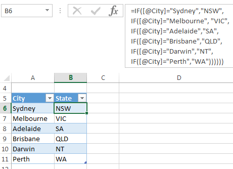
This formula uses IF to return the State for each city (I’ve wrapped each IF onto a separate row for clarity):

=IF([@City]="Sydney","NSW",
IF([@City]="Melbourne","VIC",
IF([@City]="Adelaide","SA",
IF([@City]="Brisbane","QLD",
IF([@City]="Darwin","NT",
IF([@City]="Perth","WA"))))))

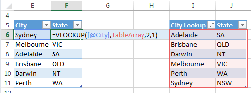
A more efficient way to return the State values is to use VLOOKUP to find the city (lookup_value) in the table_array and return the state:

Tip: For bonus efficiency points sort the city column in alphabetical order. Then you can use the VLOOKUP sorted list method i.e. use 1 or TRUE for the last VLOOKUP argument; [range_lookup]:

=VLOOKUP([@City],TableArray,2,1)

Caution: with the range_lookup argument set to 1 or TRUE you must ensure every value you want to lookup is in the table_array, because this VLOOKUP will not return an error if your lookup_value isn’t found. Instead it will return the next closest match.

An even better alternative to VLOOKUP is INDEX & MATCH. If your workbook is still slow, then replace VLOOKUP’s with INDEX & MATCH. Make sure the MATCH value is in a helper column i.e. not another nested formula.

Download the workbook

Alternatives to Multiple Nested Functions

The 22 IF whopper formula sent in by one of our members needs more than just a VLOOKUP to replace it. Unfortunately, I don’t have the data so I can’t demonstrate a solution, however I can describe the approach.

Simply put, the formula needs to be broken into separate steps:

Step 1: Insert a helper column to extract the lookup_value for each row. That is, put the AND and LEFT parts of the formula into a helper column, so you can then use VLOOKUP to find that value in the lookup table_array.

Now, I know some of you pride yourselves on not needing helper columns, but using helper columns doesn’t make you a formula amateur.

In fact, often it’s much more efficient to use a helper column than to write formulas like the one above.

Step 2: create a lookup_table that contains the lookup_values and the result you want returned. Remember, use INDEX & MATCH if VLOOKUP is still slow.

More Performance Tips

If you’re often wrangling sluggish Excel workbooks then it will pay to spend some time perusing fellow Excel MVP, Charles Williams’ website.

Charles has also developed a toolset designed to help you understand, manage and improve workbook performance. It’s called Fast Excel and includes:

Profiler - gives you a comprehensive set of tools focussed on finding and prioritising calculation bottlenecks. If your spreadsheet takes more than a few seconds to calculate you need FastExcel profiler to find out and prioritize the reasons for the slow calculation

Manager - contains tools to help you build, debug and maintain Excel workbooks.

Speed Tools - provides you with a state-of-the-art tool-kit to help you speed up your Excel Calculations

If you have performance tips please take a moment to share them in the comments below.