Formulas containing dates and time in Excel can be frustrating if you don’t understand how they work.
And even if you do they seem to work differently from one formula to another!
A few weeks ago Dave wrote to me as he was having trouble getting a SUMIFS formula to correctly use dates referenced in its criteria.
For example let’s take the data below and say we want to sum the Sale Amount if the sales person is ‘Brady’, and the dates of the sales are between 1/1/2012 and 2/2/2012.
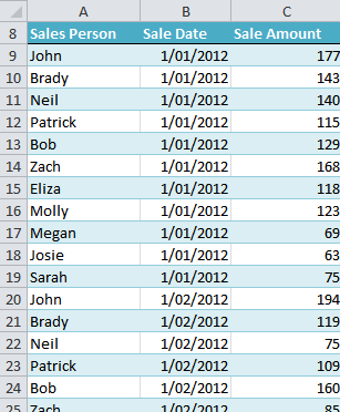
I’ve given the columns in my table the following named ranges:
- Sales Person = salesperson
- Sale Date = sales_date
- Sale Amount – sale_amt
I’ve set up my criteria at the top of my worksheet:
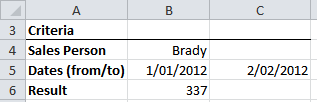
And I’ve given cells B5 and C5 range names:
- B5 = from_date
- B6 = to_date
I like to use named ranges as it makes building the formula easier and it’s more intuitive to read and interpret what the formula is doing.
SUMIFS Formula Using Date Criteria
In cell B6 I’ve put my SUMIFS formula:
=SUMIFS(sale_amt,salesperson,B4,sales_date,">="&from_date,sales_date,"<="&to_date)
Notice how the first date criterion is made up of text (surrounded by double quotes) then the ampersand, then a reference to a named range.
That’s because;
- Excel interprets the text ">=" as >=
- And the ampersand (&) tells Excel to join the text >= to the next part of the formula
Therefore the criterion ">="&from_date solves to read >=B5.
Likewise the criterion "<="&to_date solves to read <=B6.
Alternatively if you wanted to hard code the date criteria your formula would look like this:
=SUMIFS(sale_amt,salesperson,B4,sales_date,">=1/1/2012",sales_date,"<=2/2/2012")
Thanks for your question Dave.

Brilliant explanation.
Thanks a lot. 🙂
Thank you so much for explaining this formula. I looked in many other websites and it wasn’t half as clear as here … very happy I found it.
Hi Juan,
Glad that you found it useful 🙂
Regards
Phil
A B C
Jan-01-14 Potato $100.00
Jan-01-14 Onion $225.00
Jan-02-14 Carrot $300.00
Jan-02-14 Reddish $100.00
Jan-03-14 Apple $150.00
Jan-03-14 Orange $200.00
I want to sum of a given date (e.g. Jan-02-14)
Hi Buddy,
If you put the desired date in E1, and the product in F1, you can use the formula:
=SUMPRODUCT((A1:A6=E1)*(B1:B6=F1)*(C1:C6))
Catalin
Name Pieces Value
salam 2 5000
kamal 3 3000
minto 1 2000
salam 4 2000
kamal 3 1000
minto 5 3999
salam 3 5000
kamal 6 2500
minto 6 1600
salam 4 1500
kamal 3 1200
salam 4 2700
minto 2 3800
salam 1 7000
kamal 2 4100
salam 3 500
I want to sum salam & kamal values in one cell. so what formula use?
Hi Mohammad,
You can try this:
=SUMIF(A2:A17;”salam”;C2:C17)+SUMIF(A2:A17;”kamal”;C2:C17)
Catalin
You are great!
I repent the time I wasted trying to use the “>” sign with cell reference in criteria to compare a date before visiting your site. Thanks for the tip and trick… 🙂
🙂 You’re welcome, Tariq.
Thank you so much for the explanation of sumifs with dates as criteria.
Microsoft is really a crappy company…
– nothing about this is given in the help online (they keep repeating the same simple examples that add nothing to a more complex problem)
– inconsistent with other functions like ‘If’ where you can write: IF(G39>D51,0,1) and it works very well when G39 and D51 are dates. Excel can handle the comparison of dates directly without having to write =IF(G39&”>”&D51,0,1)
Excel is been made by lousy programmers who never use it or test it…
Hi Francois,
Thanks for sharing your feelings (frustrations) with Excel. I used to get confused with what appears to be inconsistent requirements for date handling too, which is why I wrote this tutorial.
Kind regards,
Mynda.
Dear Mynda
Thank you so much for the explanation of using logical operators (>, <= etc) in the SUMIFS. I had a particular case where I wanted to count the number of times a customer number occur in a dataset, IF it matches 2 conditions. One of these conditions was that the DATE must occur within 90 days of the other occurence(s). I applied your knowledge shared here, in a COUNTIFS statement, and it worked beautifully. Thank you so much.
Best regards
Sarel
🙂 You’re welcome, Sarel. Glad I could help.
Can we write a SUMIF/S criteria that include a calculation. I have a 2 column table on one work sheet (WS1) and another 2 columns on another worksheet (WS2). All of them are formated as number. my goal is to fill up WS2!B column based on other data. For example WS2!B2 value is equal to sum of numbers in WS1! B column which their WS1! A value at the same row meet the following criteria:
Sin (WS2! $A$2)-Sin (WS1! A*)<0.2
the result will be shows at WS2! B2. and for WS2! B3 criteria would be:
Sin (WS2! $A$3)-Sin (WS1! A*)<0.2
Thanks,
Hi Omid,
Greetings.
It’s good to have you here. Let’s get down to your concerns.
First, what do you mean by calculation? If you mean a formula within a SUMIF, then I don’t think you can
have a formula within a SUMIF. We might as well use SUMPRODUCT.
Second, when you describe your problem, It seems afterall that you don’t need SUMPRODUCT or a SUMIF.
What you need is a simple IF to return the value in B column from WS1 to the B column of WS2:
Assumptions: You are in sheet 2 to write the formula for col B.
WS1 Data
—A—- —B–
1- 12…….10
2- 02…….20
3- 03…….30
4- 04…….40
WS2Data
—A—- —B–
1- 0……..see formula below & copy it down
2- 02…….
3- 03…….
4- 04…….
=IF((SIN('WS1'!A1)-SIN(A1))<0.2,'WS1'!B1,0)This will return or list as you say the value of B col from WS1 to B of WS2.
IF the SIN of A of WS1 - SIN of A WS2 < .2 then return it to WS2 B Column Else return ZERO(0) Just in case you really needed a sumproduct it will only need one cell to add a column for example column A in WS2:
=SUMPRODUCT((A1:A4)*((SIN('WS1'!A1:A4)-SIN(OmidWS2!A1:A4))<.2))Please do send your file for further clarifications here: HELP DESK.
We are more than willing to help.
Please read our very informative blogs:
SUMPRODUCT
IF FUNCTIONS
SUMIF
Cheers.
CarloE
madam,
Good day!
Thank you for very much, I really appreciate all the information and help you have done.
More power to you and God bless,
Jobet
Thank you, Jobet 🙂