Referencing the Next Row in Power Query

Unlike Excel, referencing the next row in Power Query, or even the previous row, is not as simple as we Excel users have become accustomed.

There are several approaches, but some are more efficient that others, which is something to consider if you’re working with a lot of data. Let’s take a look.

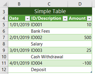
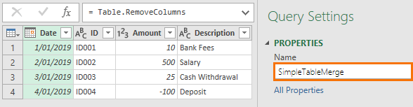
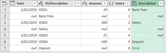
First, the data. Below I have a simple table that contains transaction data with the description on the row below each transaction. I need to bring the description up to the row above and then remove the rows that only contain the description.

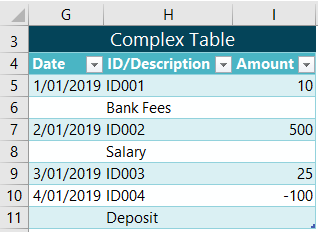
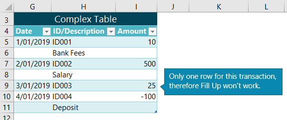
Thankfully the table above has a consistent pattern that I can exploit. However, sometimes we have a table that has an inconsistent pattern, like the one below where ID003 on row 9 doesn’t have a description:

We’ll look at solutions for the Simple Table first, then move on to the Complex Table.

Download Workbook

Referencing the Next Row in Power Query – Simple Table

Option 1: Fill Up

One way we can bring data form one row up to the row above is with the Fill Up tool.

Step 1: Load data to Power Query

My data is formatted in an Excel Table called ‘SimpleTable’, so I’ll use the ‘From Table/Range’ connector of the Data tab of the ribbon:

Note: Excel 2010 and 2013 users will go to the Power Query tab > From Table/Range.

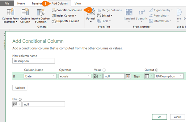
Step 2: Add Conditional Column

We’ll use an ‘if’ statement to determine whether the row contains the transaction or the description. If it contains the description, we’ll bring it across to the new column, otherwise we’ll leave it blank (i.e. null).

The Date column contains a null value where there is a description, and we’ll use this for our logical test. Using the dialog box it’s easy to build a conditional if statement:

Step 3: Fill Up

We can now use the Fill Up tool to bring the descriptions up to the row above. Select the new Description column > Transform tab > Fill > Up:

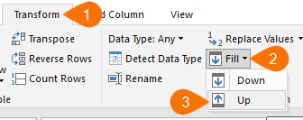
Tip: If you want to reference the row above, then you could use Fill > Down to copy the data down to the next row.

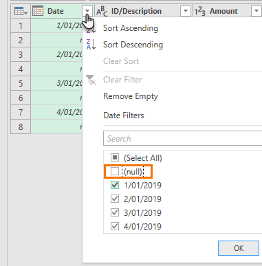
Step 4: Remove null rows

Let’s remove the rows we don’t need. Click on the drop down on the Date column > deselect ‘null’ from the list:

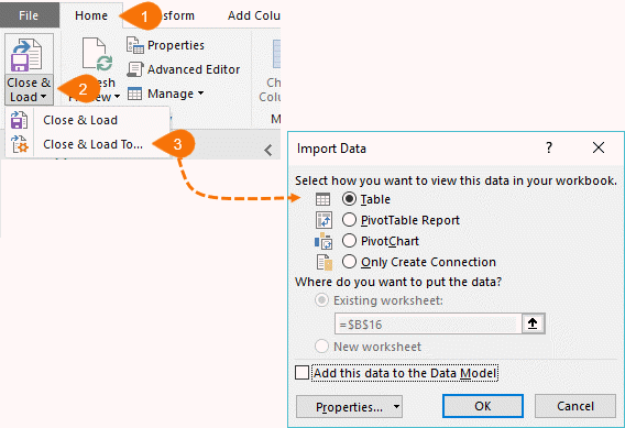
Step 5: Close and Load

Now you're ready to load the data to a Table in the workbook, the Data Model (Power Pivot), or for later versions of Excel you can jump straight to a PivotTable or PivotChart:

Option 2: Duplicate Query and Merge

Step 1: Load Data to Power Query

As shown in step 1 of Option 1.

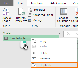
Step 2: Duplicate the Query

Right-click the query name in the Queries pane > Duplicate:

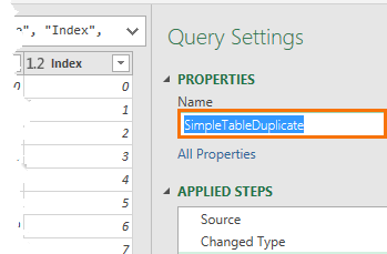
Step 3: Rename the Duplicate Query

In the Query Settings > Properties rename this query ‘SimpleTableDuplicate’:

Step 4: Add an Index Column to both queries:

Back in the SimpleTable query go to the Add Column tab > click on the ‘Index Column’ drop down > From 1:

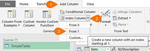
Then go to the SimpleTableDuplicate query and add an index column ‘From 0’.

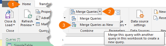
Step 5: Merge Queries

On the Home tab > Merge Queries > Merge Queries as New:

In the Merge dialog make the following selections from the drop down lists, then hold the CTRL key while left clicking the Index columns in each query:

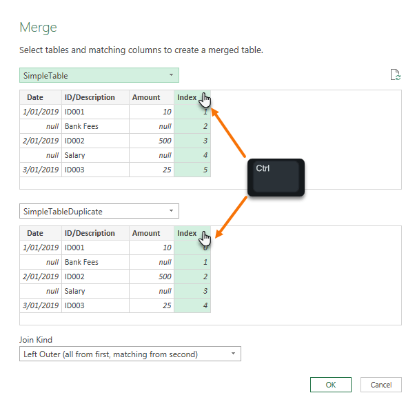
Tip: If you want to bring the data down to the next row you could switch the Index in the SimpleTable to start at zero and the index in the SimpleTableDuplicate to start at 1.

Step 6: Expand the Table

Click on the double-headed arrow on the SimpleTable column:

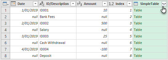
Choose the 'Expand' radio button and deselect ‘Use original column name as prefix’:

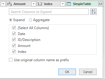
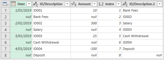
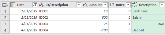
You should now have a table like this:

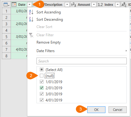
Step 7: Remove null rows

Click on the drop down on the Date column and deselect ‘null’ from the filter.

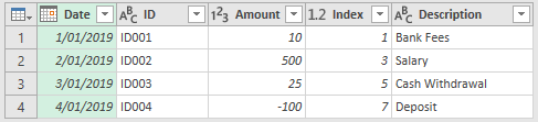
Step 8: Rename Columns

Double click the column headers for ID and Description and type in new names like so:

Step 9: Delete the Index Column

The index column has done its job. Click the column header and press the Delete key to remove it.

Step 10: Rename the query

Step 11: Close and Load

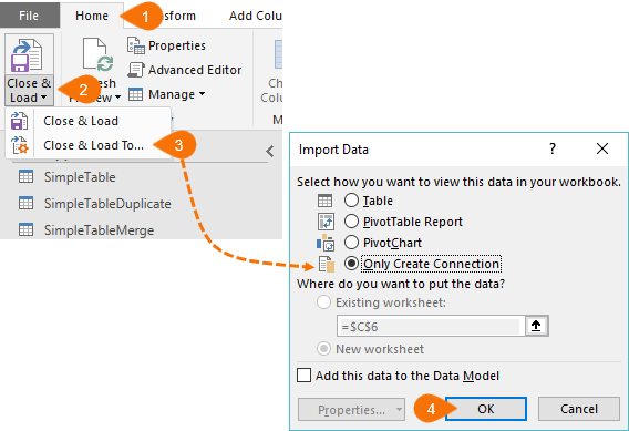
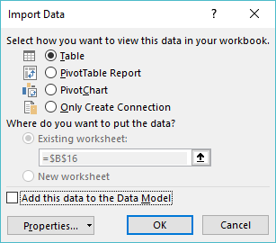
You should now have 3 queries; SimpleTable, SimpleTableDuplicate and SimpleTableMerge. You’re ready to Close & Load, but we only want to load one table; SimpleTableMerge. Go to the Home tab > Close & Load > Close & Load To… > in the ImportData dialog box choose ‘Only Create Connection’:

Step 12: Change Load to Settings

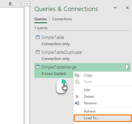
In the Queries & Connections pane on the right-hand side of the worksheet > right-click ‘SimpleTableMerge’ query > Load To…

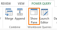
Note: If you can’t see the Queries & Connections Pane you can turn it on via the Data tab. For Excel 2010 and 2013 users you can turn it on via the Power Query tab > Show Pane:

In the dialog box you can choose where you want to load the data (note, earlier versions of Excel will not have all of the options shown below):

Ok, that seems like a lot of work, but I think you’ll agree that it’s all very straight forward.

Option 3: Custom Function

If you find you have performance issues with options 1 and 2 then you might like to try Imke Feldman’s custom function. It’s an advanced technique that creates a table from a list of columns and then duplicates the table shifting it down one row before joining them together.

I’ve included a modified version of it in the workbook you can download above. You’ll see the queries are called fnSimpleTableShiftedList and SimpleTableShiftedList. You can learn how it works here on Imke’s blog.

Referencing the Next Row in Power Query – Complex Table

The complex table requires a different approach because it doesn’t have a consistent pattern we can exploit. Here it is again for reference:

Step 1: Load Data to Power Query

As shown in step 1 of Option 1.

Step 2: Add Index Column

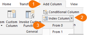
In the ComplexTable query go to the Add Column tab > click on the ‘Index Column’ drop down > From 0:

Step 3: Add Custom Column

In this step we’re going to use the Index column to reference the row below if the Amount column contains ‘null’.

Add Column tab > Custom Column. In the Custom Column dialog box enter the following formula (note: Power Query is case sensitive):

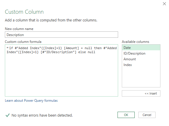
= if #"Added Index"{[Index]+1} [Amount] = null then #"Added Index"{[Index]+1} [#"ID/Description"] else null

In English it reads:

Use the Index column to move down +1 row from the current row and reference the Amount column to check if the value is null. If it is, return the value from the ID/Description column 1 row down from the current row, otherwise return null

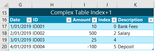
The formula returns a new column called ‘Description’:

Step 4: Filter null rows

Click on the drop down on the Date column and deselect ‘null’ from the filter. The result should look like this:

Step 5: Close & Load

And finally, Close & Load to a table or the Data Model.

Learn More Power Query

Power Query is an amazing tool that allows use to automate the gathering and cleaning of data resulting in huge time savings. If you'd like to learn how to use it, please consider my Power Query course to fast track you there.