How to Compare Two Excel Sheets and Find Every Difference

Your colleague sends you an updated version of a file you built last week. You open it and everything looks fine at first glance.

Then the doubt creeps in.

Did they change the numbers? Move a row? Fix something or break something?

You start scanning both versions. Your eyes jump back and forth between sheets. Five minutes later, you still are not confident you caught everything.

This is a common problem in Excel. Comparing two versions manually is slow, error-prone, and frustrating.

In this guide, you will learn three reliable ways to compare Excel sheets and find every difference. You will also learn why Excel sometimes shows cells as identical when they are actually different.

Watch How to Compare Two Excel Sheets

Get the Example File

Step 1: View Both Excel Sheets Side by Side

Before comparing anything, you need to see both sheets at the same time.

If both sheets are in the same workbook:

1. Go to the View tab
2. Click New Window
3. Go back to View
4. Click Arrange All
5. Choose Vertical and click OK

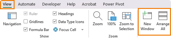
You now have two windows of the same workbook.

In one window, select Version 1. In the other, select Version 2.

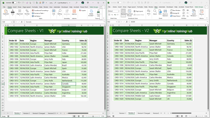
If your sheets are in separate workbooks, simply open both files and use View > Arrange All > Vertical.

This setup alone can make manual comparison easier, but it is not enough for accuracy.

Method 1: Compare Excel Sheets Using Conditional Formatting

This is the fastest way to visually highlight differences between two sheets.

How to set it up

1. Select the data range in Version 1
2. Go to Home > Conditional Formatting > New Rule
3. Choose “Use a formula to determine which cells to format”
4. Enter this formula, make sure both references are relative, not absolute:

=C5<>'Version 2'!C5

5. Set a format such as red font with a light fill
6. Click OK

Excel will instantly highlight every cell that does not match.

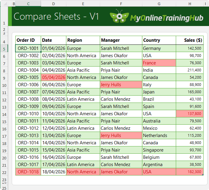
When to use this method

• Your data structure is identical
• Rows and columns are aligned
• You want a quick visual check

This method is fast and effective, but it has a limitation.

The Hidden Differences Problem in Excel

Sometimes two cells look identical, but Excel still flags them as different.

This is not a bug. It is Excel doing exactly what it should.

Here are the three most common causes.

1. Trailing spaces

A value like “France ” contains an invisible space at the end. You cannot see it, but Excel counts it.

2. Numbers stored as text

A value that looks like 43100 may actually be stored as text. Excel treats it differently from a true number.

3. Dates stored inconsistently

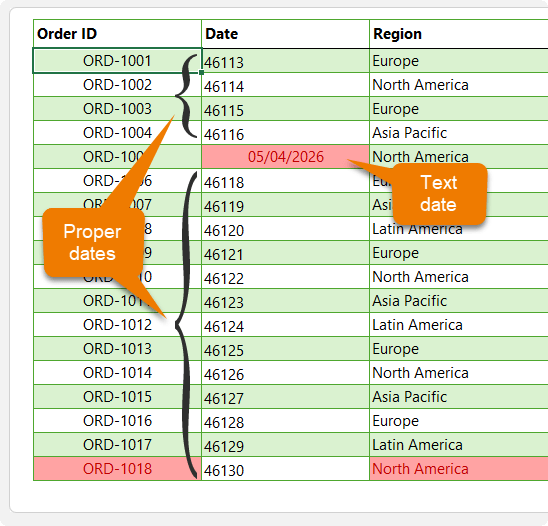
Two cells may both display 05/04/2026, but one is a real date and the other is text.

They look the same but behave differently.

How to Detect Hidden Differences

Check for trailing spaces

Use the LEN function to take the length of one cell from the other:

=LEN(G5)-LEN('Version 2'!G5)

If the result is not zero, the values are not identical.

Check for numbers stored as text

Look for the green error indicator in the cell.

Hover over the indicator to convert to a number.

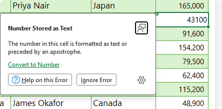
Check for text-based dates

Press Ctrl + ` to toggle formula view.

Real dates will show as serial numbers. Text dates will still look like dates.

Method 2: Create an Excel Audit Sheet (Change Log)

If you need a clear record of changes, this method is far more useful than simple highlighting.

You will build a third sheet that shows both old and new values side by side.

Step-by-step

1. Insert a new sheet and name it Change Log
2. Add your column headings
3. Enter this formula:

=IF('Version 1'!C5='Version 2'!C5,
'Version 2'!C5,
"V1: "&'Version 1'!C5&", V2: "&'Version 2'!C5)

4. Copy the formula across your dataset

What this does

• If values match, it shows the value
• If values differ, it shows both versions clearly

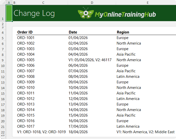
Example output as seen in the screenshot below in cell D9:

V1: 05/04/2026, V2: 46117

Note: the correctly formatted date displays as the date serial number.

When to use this method

• You need a clear audit trail
• You want to share changes with others
• You need context, not just highlights

This approach turns your comparison into a report.

Method 3: Compare Excel Data Using Power Query

The first two methods work well when your data lines up perfectly.

They break down when:

• Rows are added or removed
• Data is sorted differently
• Records shift position

Power Query solves this by comparing records, not positions.

Why Power Query is better for complex comparisons

Instead of comparing cell by cell, Power Query matches rows.

This allows you to identify:

• New records
• Deleted records
• Changed records

Step-by-step overview

1. Convert both datasets into Excel Tables using Ctrl + T
2. Name them Version1 and Version2
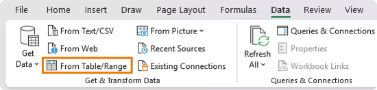
3. Load into Power Query using Data > From Table/Range

4. Home tab > Close & Load To > Only Create Connection
5. Repeat the Power Query steps for the Version 2 table.

Compare Version 1 against Version 2

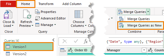
1. Open the Power Query editor
2. Select Version1 query
3. Select Merge Queries as New

4. Choose Version2 as the second table
5. Select all columns to match holding CTRL
6. Choose Left Anti join

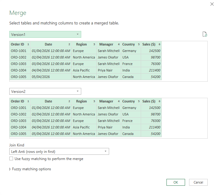
This returns rows that exist in Version1 but not in Version2.

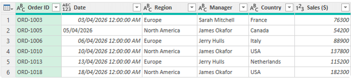
Compare Version 2 against Version 1

Repeat the process:

• Use Version2 as the base
• Choose Version1 as the second table
• Select Left Anti join

This returns rows that are new or changed in Version2.

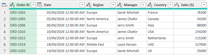
Load results

Load both queries back into Excel as tables.

The real advantage

When your source data changes:

1. Add new data
2. Go to the Data tab > Refresh All

Your comparison updates automatically.

No rework required.

Which Method Should You Use?

Use Conditional Formatting when you want a quick visual comparison.

Use an Audit Sheet when you need a clear record of changes.

Use Power Query when your data changes frequently or does not align perfectly.

If you are working with real-world datasets like customer lists, product data, or transaction logs, Power Query is usually the most reliable option.

Final Thoughts

Comparing Excel sheets manually is not just slow, it is risky.

Small differences are easy to miss, especially when data looks identical but is not.

These three methods give you a structured way to find every difference with confidence.

Start with conditional formatting for quick checks.

Move to an audit sheet when you need clarity.

Use Power Query when accuracy and scalability matter.

If you want to go further with automation, check out my Power Query course and transform repetitive workflows into a one-click process.