Imagine that you are preparing data for a pivot table, and you want to make sure that all the cells contain the correct data type.
We know that a date or number entered as text can mess things up so if we had a quick way to identify these problems, it could save a lot of time and effort.
This VBA routine allows us to quickly identify such issues.
Source Data
We have data laid out like this, and everything looks ok.
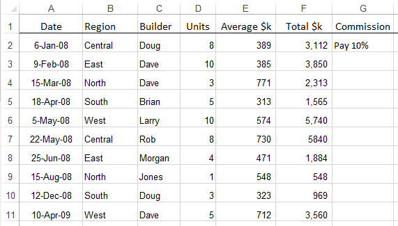
But, some of those dates are actually text, and so are some of the numbers.
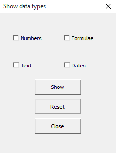
The VBA color codes each of the data types differently so you can easily see where the problems are.
- Numbers are light blue
- Formulae are yellow
- Text is green
- Dates are mid-blue
How the Code Works
The VBA uses the SpecialCells method to create a range object for each of the groups of cells containing formulae, text and numbers.
As dates are numbers in Excel, the numbers range contains both what we would consider numbers, and dates.
By using the Areas property of each of these ranges, we can set the background color, which in VBA is the cell's Interior.ColorIndex, to a color of our choosing.
I've created a form to allow the user to check which type of data they want highlighted. If a check box is checked, that data type is highlighted. If the check box is not checked, then cells containing that corresponding data type has no background color. I've included a Reset button to allow users to quickly clear all check boxes and cell colors.
For this demonstration I've run the macro from a shape on the sheet, but it would be more useful to store it in your PERSONAL.XLSB and then run it from the Ribbon or QAT.
It's always a good idea to create a copy of your data before working on it like this, if for nothing other than you will lose any colors you have applied to cells.
Choosing Colors for Highlighting
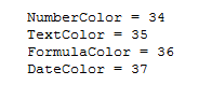
Colors are specified by numeric values, and I used David McRitchie's post on the Excel color palette to choose mine.
I've hard coded the values into four variables, and tried to choose ones that won't burn your eyes.
You can of course choose your own colors.
A nice enhancement would be to use a color picker on the form, but I think this is another blog topic.
Acknowledgement
I found code by John Walkenbach to create a worksheet map and what I have written here is based on that.
Sample Code
Enter your email address below to download the sample workbook.
You can download a sample workbook containing this code.


Wonderful code! Great tool for troubleshooting! From my testing, if all four items are checked in the form, and if the worksheet does not have one of the types (such as formula), then the routine errors out. This is not a major issue, since the macro can then be rerun without the formula box being checked – but it would be nice if the macro worked fully the first time.
Thanks again Phil for your great work!
Thanks Paul,
You shouldn’t get that error as I fixed the code to prevent this happening. You must have an older copy of the workbook. Please download it again and let me know if you are still getting those errors.
Regards
Phil
one can add select constants / formulae (and comments / data validation / conditional formatting) to the QAT by going to Editing/Find&Select on the Home ribbon and right clicking the desired option
nothing to undo and no VBA (and no date selection nor automatic shading, but shading’s only another click away and constants that are dates can be selected by using ctrl-F, “/” , Find All, ctrl-A)
not nearly as elegant as Simon but still effective
Hi Jim,
Thanks for pointing out an alternative. I personally don’t like that I have to de-select the found cells every time before selecting the next lot though!
There’s no distinction between text, dates and numbers either but I guess it’s horses for courses and whatever works best for you.
Regards
Phil
sorry, for Simon read Phil (the other variety of Treacy works here!)
🙂 no worries
Another useful tool, Phil. I’ve previously used a similar approach but the result was achieved via Conditional Formatting functionality – your macro is much easier.
I gather that the target range includes ALL used cells on the active sheet. If so, how can your code be adapted to target only a user selected range – by changing “ActiveSheet” in each iteration of “With ActiveSheet.Range(Area.Address)” to “Selection”?
Thanks Col.
Yes the original macro will include all cells on the sheet. To just work with a selection of cells you need to change 3 lines of code.
At the top of the ShowDataTypes sub, you’ll see these lines where the various ranges that the routine uses are set
Set FormulaCells = Range("A1").SpecialCells(xlFormulas, xlNumbers + xlTextValues + xlLogical)
Set TextCells = Range("A1").SpecialCells(xlConstants, xlTextValues)
Set NumericCells = Range("A1").SpecialCells(xlConstants, xlNumbers)
change these to
So we are just changing Range(“A1”) to Selection
Cheers
Phil
I have downloaded the sample workbook, stored it but the Show Data Types button doesn’t run the macro (I have enabled macros in the Trust Center). What is my problem?
Hi Frank,
When you say you have enabled macros in the Trust Center, do you mean you have it set to the ‘Enable all macros (not recommended; potentially dangerous code can run)’ setting? That’s the only setting in the TC that allows macros to run.
In the Trust Center a better setting is ‘Disable all macros with notification’. When this workbook is then opened, you should be prompted to enable the macros in it.
Phil
Great idea, nicely packaged
I use a similar technique to highlight which numbers have been updated from a default value
Defaults are formulae that can be overwritten with a number
I have a defined name IsFormula = GET.CELL(48,INDIRECT(“rc”,)) and then use that with conditional formatting to make bold any of the target cells that are no longer a formula
It’s not totally foolproof but it does what I need it to (NB needs saving as xlsm)
I think I might have done this with a little help from JW too
Thanks for this Jim.
Phil