Excel PivotTable Calculated Items by Position

• Share on Facebook.
• Share on Twitter.
• Share on Google+
• Share on LinkedIn
• Pin It!

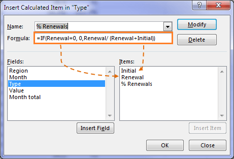
A while back I wrote about how to create Excel PivotTable Calculated Items using the conventional approach of referencing the item name in the formula like this:

But did you know you can also refer to items by their position in the PivotTable relative to the column containing your Calculated Item?

Download the Workbook

Referencing Excel PivotTable Calculated Items by Position

For example, let’s say we have some data by month like so:

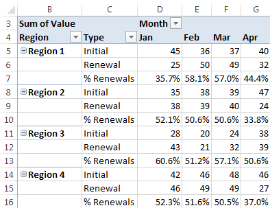
And in column H we want to add a Calculated Item for the rolling average of the last 3 months. In our formula we can reference ‘Apr’ with Month[-1], Mar with Month[-2] and so on. The minus sign tells Excel that the Month column is to the left of our Calculated Field.

Inserting a Calculated Item for Rolling Average

To insert a PivotTable Calculated Item for the rolling 3 month average:

1. Select a cell in the column labels area of the PivotTable. E.g. click on cell G4 containing ‘Apr’.
2. Then on the PivotTable Options tab (Excel 2010), or PivotTable Analyze tab (Excel 2013) > Fields, Items & Sets > Calculated Item. This opens the dialog box below:

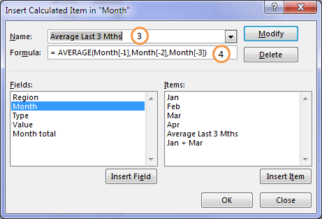
3. Give your new Item a name
4. Enter your formula; remember I want to AVERAGE the last 3 months, so I will reference the Field name ‘Month’ and in square brackets I’m telling Excel the position of the columns I want it to use relative to the column containing my new Item. So my formula is:

= AVERAGE( Month[-1], Month[-2], Month[-3])

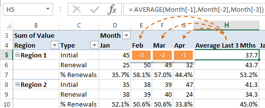
In the image below you can see that Month[-1] is referencing ‘Apr’ as this is the Month column that is one back from the column containing my Calculated Field in column H:

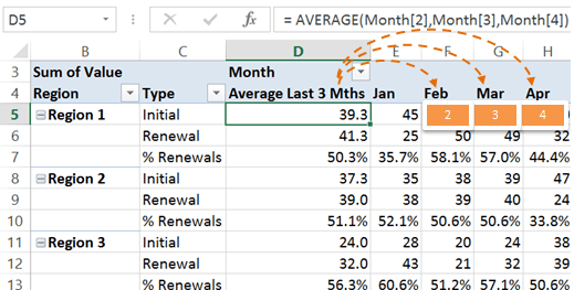
Alternatively if the position of the ‘Average Last 3 Mths’ column was before ‘Jan’ my formula would be:

=AVERAGE(Month[2], Month[3], Month[4])

Referencing Items by Position Gotchas

• High Maintenance: The above formula with the Average to the left of the data is high maintenance because as new months are added the position of the last 3 months changes relative to the column containing the formula.

  For example, if we added May data then we’d need to edit the formula so that it picked up Month[3], Month[4], and Month[5].

  And before you ask…no you can’t use dynamic ranges in PivotTable Calculated Field/Item formulas 🙂

  I therefore prefer to position of the Last 3 Months column to the right of the data, but that’s not bullet proof either as you’ll see in my next point.

• Drag & Drop: Putting the ‘Last 3 Months’ column to the right of the month columns doesn’t make it maintenance free. You still have to update it as new months are added because they will be added after your Calculated Item column (as you can see below with ‘May’ being added in column I), but it’s a simple case of dragging the ‘Average Last 3 Months’ column to the end of the PivotTable….just don’t forget to do this!

• Filters: Items referred in this way can change whenever the positions of items change or different items are displayed or filtered. Filtered items are not counted in this index.
• Errors: If the position that you give is before the first item or after the last item in the field, the formula results in a #REF! error.

Use with Caution

So as you can see, referencing Excel PivotTable Calculated Items by Position is a great way to calculate rolling averages, or rolling totals, but you must remember to maintain them or you could end up with some kooky data.

Please Share

If you liked this or know someone who could use it please click the buttons below to share it with your friends on LinkedIn, Google+, Facebook and Twitter.